

Yes. If you embed records with a model that places similar items close together, an anomaly is a record whose neighborhood is unusually empty: its nearest “normal” neighbors are far away, or there are very few of them within a fixed radius. A vector database turns that idea into a repeatable service. You store embeddings of a reference population, query each new record for its k nearest neighbors, and turn the distances into a score that sends the most unusual cases to a reviewer. The score ranks candidates for investigation. It is not a calibrated probability that something is broken, and it is only as good as the embedding and the reference set behind it.
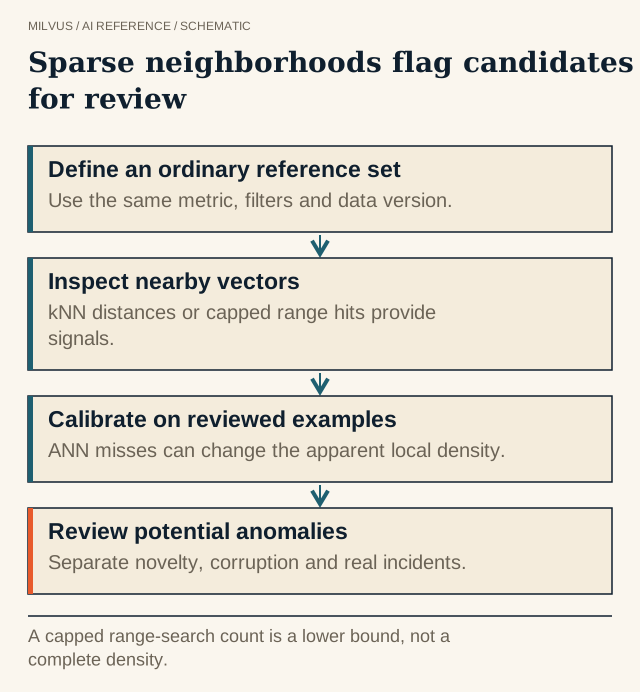 Sparse neighborhoods flag candidates for review. A capped range-search count is a lower bound, not a complete density.
Why do nearest-neighbor distances expose anomalies?
Distance-based detection rests on a simple assumption: normal data is dense, and unusual data sits in sparse regions of the embedding space. Four scores come up again and again:
| Score | How it is computed | Strength | Weak spot |
|---|---|---|---|
| k-th NN distance | Distance from the record to its k-th nearest reference neighbor | Simple, few assumptions, strong on deep-learning features | One global threshold struggles when clusters have very different densities |
| Mean kNN distance | Average distance to the k nearest neighbors | Less sensitive to a single lucky neighbor | Same density problem |
| Local Outlier Factor (LOF) | Ratio of the neighbors’ local density to the record’s own density | Handles clusters of different tightness | Scores are relative ratios with no universal cut-off; costlier to maintain |
| Neighbor count in radius | How many reference points fall within distance r | Maps directly to a range query | Radius must be tuned per population |
The research record backs the simple options. Sun et al. (ICML 2022) showed that the k-th nearest-neighbor distance on normalized deep features is a strong, assumption-free detector for out-of-distribution inputs, beating parametric Mahalanobis-style baselines on ImageNet-scale benchmarks. PatchCore applied the same idea to industrial inspection: it keeps a memory bank of embeddings from defect-free product images and flags image patches whose nearest stored patch is far away. Both are, at their core, nearest-neighbor lookups against a curated reference set, which is exactly the workload a vector database is built for.
The other lesson from that literature is that the representation matters more than the scoring rule. The same kNN detector can look excellent on one embedding model and mediocre on another, so model choice and evaluation belong in the design from day one.
What does the end-to-end architecture look like?
A practical anomaly-discovery system has six stages:
- Ingest and embed. Convert each record (log line, transaction, image, sensor window, document, driving clip) into a vector with a model suited to the modality. Normalize vectors if you plan to use cosine similarity, and record the model name and version alongside each vector. See how to choose an embedding model and how to build a scalable embedding pipeline.
- Define and index the reference population. Store embeddings of records you consider normal, tagged with the context that defines "normal": device type, region, customer, time window, operating mode.
- Query neighbors. For each new record, retrieve its k nearest neighbors from the matching reference group only.
- Score and threshold. Convert the distances into a score and compare it with a threshold calibrated on held-out normal data.
- Review and feed back. Send the top-scoring cases to a human or a downstream classifier, and write the verdict back as metadata.
- Evaluate and recalibrate. Track how many flagged cases turned out to be useful, and refresh the reference set and threshold on a schedule.
How do you implement it in Milvus?
Schema. Store the embedding in a FLOAT_VECTOR field, plus scalar fields for the context you will filter on (for example reference_group, sensor_id, source_system, event_time) and a review_label field you can update after review. If most queries are scoped to one group, declaring reference_group as a partition key (is_partition_key=True) lets Milvus prune the search to the partitions that hold that group instead of scanning everything. For other fields you filter on often, an INVERTED scalar index keeps filters fast.
Neighbor query. A plain top-k search with a filter gives you the distances you need for kNN scoring. Pass many query vectors in one call to score a batch:
res = client.search(
    collection_name="events",
    data=batch_vectors,                 # many query vectors per call
    limit=10,                           # k
    filter='reference_group == "night_urban" and review_label != "anomaly"',
    output_fields=["source_system", "event_time"],
)
# score = distance to the 10th neighbor (or the mean of the 10)
Two details trip people up. First, if the record being scored is already in the collection, it will be its own nearest neighbor at distance zero, so exclude it by primary key in the filter or request k+1 results and drop the self-match. Second, excluding known anomalies from the reference set (the review_label filter above) stops past incidents from making similar future ones look normal.
Range search for density. Milvus range search adds radius and range_filter to the search parameters and returns only neighbors inside a distance band. For L2 the band is range_filter <= distance < radius; for COSINE and IP, where larger means more similar, it is radius < score <= range_filter. That supports a “neighbor count in radius” signal, with two caveats. Range search returns at most limit hits, and only neighbors the ANN index actually visits, so the count is a lower bound, not a complete density measurement. Use it as a sparsity test: set limit to a small cap such as 20, and flag a record when it returns far fewer hits than ordinary records do under the same index and search parameters. A record that hits the cap is simply "dense enough"; its true count is unknown. Range search finds what is near a query, not what is far, so use it to measure sparsity around each record rather than expecting it to return outliers directly. See when to use range search instead of top-k.
Metric and index. Pick the metric your embedding model was trained for; cosine on normalized vectors is the common default (see how cosine, IP, and L2 differ). Approximate indexes such as HNSW occasionally miss a true neighbor, which slightly inflates kNN distances. Calibrate your threshold with the same index and search parameters you run in production, so that bias is baked into the baseline rather than showing up as false alarms.
How should you set thresholds?
Distances have no meaning in the abstract. A cosine distance of 0.3 can be routine for one model and alarming for another. Calibrate empirically:
- Hold out a sample of known-normal records from each reference group, score them against the rest, and set the threshold at a high percentile of that distribution (for example the 99th or 99.5th), sized to the number of alerts your reviewers can handle each day.
- Keep separate thresholds per group when densities differ. A tight cluster of identical server logs and a loose cluster of free-text support tickets should not share one cut-off.
- Recompute the baseline on a schedule by re-scoring a fresh sample, and change the reference set deliberately with a version tag. Letting thresholds drift silently as new data arrives is how slow-moving problems become “normal.”
How do you separate real discoveries from noise?
High scores have several causes, and only some are interesting:
- Broken inputs. Empty text, corrupted images, or failed embedding calls often produce vectors far from everything. Route records that fail validation to a separate data-quality path before scoring, or they will crowd the review queue.
- Wrong reference population. A rare-language document looks odd in a mostly English corpus without being defective. A night-time driving clip is far from daytime examples, yet it should be compared with other night clips. Scoping by group fixes most of these.
- Irrelevant variation. A camera firmware change or a new log format can shift embeddings without any real-world event. Keep source metadata so an analyst can tell a pipeline change from a genuine rare case.
- Genuine novelty. These are the records worth labeling. Show reviewers the record next to its nearest neighbors, which is cheap to retrieve and usually explains the score faster than the number itself.
Combine the vector signal with structured rules where it helps. Hard filters (exclude known-faulty sensors, restrict a scan to one deployment) and simple thresholds on numeric fields catch problems that embeddings blur.
How do you know the system works?
Build a labeled set of important rare cases and ordinary variations, then measure what matters for a review team: precision among the top N alerts, recall of known incidents at your alert budget, and AUROC if you want a threshold-free comparison across embedding models. Always compare with a random or stratified sample of the same size; if reviewers find nearly as many useful cases by random sampling, the scoring is not earning its keep. Re-run the evaluation when the model, the data source, or the reference set changes. The same retrieval-quality ideas apply here as in search, covered in how to evaluate retrieval quality.
Neighborhood search also works in reverse. Once you have a few confirmed anomalies, use them as queries to find similar unlabeled records, which turns one reviewed incident into a cluster of candidates. Related techniques for picking representative or underrepresented data are covered in diversity sampling with embeddings and document clustering with embeddings.
Where does this pattern fit?
Embedding-based anomaly discovery suits data where rules are hard to write but “looks unlike the rest” is a useful signal: unusual log or trace patterns, odd transactions or account behavior, defects in product images, rare driving scenarios in autonomous-vehicle fleets, and out-of-distribution inputs reaching a deployed model. It is weaker for anomalies defined by a single numeric threshold, where a plain rule or time-series detector is simpler and more transparent.
To try it, load a sample of your data into Milvus with the Quickstart, score a held-out set with top-k search, and inspect what lands at the top. The Milvus Bootcamp has runnable application examples to start from.
Sources and further reading
- Milvus: Range search
- Milvus: Filtered search
- Milvus: Use partition key
- Milvus: Metric types
- Milvus: Build RAG with Milvus
- Sun et al., Out-of-Distribution Detection with Deep Nearest Neighbors (ICML 2022)
- Roth et al., Towards Total Recall in Industrial Anomaly Detection (PatchCore)
- Local outlier factor (Wikipedia)
- Sentence Transformers: clustering embeddings


