

Cosine similarity, inner product (dot product), and Euclidean (L2) distance are three ways of scoring how close two embedding vectors are. Cosine compares only direction, inner product rewards both direction and length, and L2 measures the straight-line gap between the two points. For unit-length vectors all three produce the same ranking; for unnormalized vectors they can disagree, so the right choice is the one your embedding model was trained with.
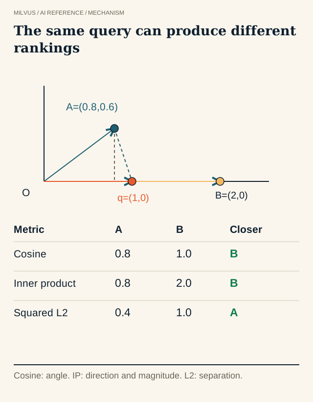 Angle, projection, and distance can produce different rankings
Cosine vs. dot product vs. Euclidean at a glance
For a query vector q and a stored vector d:
| Cosine similarity | Inner product (dot product) | Euclidean distance (L2) | |
|---|---|---|---|
| Formula | (q · d) / (‖q‖ ‖d‖) | q · d = Σ qᵢ dᵢ | √Σ (qᵢ − dᵢ)² |
| What it measures | Angle between the vectors | Projection of one vector onto the other, scaled by both lengths | Straight-line separation |
| Sensitive to vector length? | No | Yes | Yes |
| Range | −1 to 1 | Unbounded | 0 to ∞ |
| Better match | Higher | Higher | Lower |
| Typical fit | Text and sentence embeddings, models trained with a cosine objective | Models trained with a dot-product objective, recommendation embeddings where length carries signal | Clustering, image and feature vectors, models trained with an L2 objective |
Milvus metric_type | COSINE | IP | L2 |
Two details in this table catch people out. First, inner product and cosine are similarity scores, not distances in the mathematical sense: they grow as vectors get closer, and inner product does not satisfy the triangle inequality. With unnormalized vectors, a document’s best inner-product match is not even guaranteed to be itself, because a longer vector pointing roughly the same way can outscore it. Second, Milvus reports L2 as the squared distance, skipping the final square root. Ranking is unchanged because the square root is monotonic, but any threshold you set must be in squared units.
How each metric works
Cosine similarity divides the dot product by both vector lengths, which leaves only the cosine of the angle between them. A score of 1 means the vectors point the same way, 0 means they are orthogonal, and −1 means they point in opposite directions. Because length is divided out, doubling a vector does not change its score. That makes cosine a natural fit when length is an artifact (longer documents, different token counts) rather than meaning. It is undefined for a zero vector, so pipelines should reject or handle empty inputs explicitly.
Inner product is the plain sum of element-wise products. Geometrically it equals ‖q‖ ‖d‖ cos θ, so it combines alignment with magnitude. That is useful when a model deliberately encodes something in length. In recommendation systems trained on interaction data, for example, frequently consumed items often end up with longer embeddings, and a dot-product score lets that popularity influence ranking. If you do not want that effect, normalize or switch to cosine. Inner product is also the cheapest of the three to compute, which is one reason many systems normalize once at ingestion and then score with IP.
Euclidean distance treats each vector as a point and measures how far apart they are. It responds to differences in both direction and length, and it is the familiar distance behind k-means and many clustering methods. It is a true metric, so it behaves the way geometric intuition expects.
A worked example where the rankings disagree
Take a query q = (1, 0) and two stored vectors: A = (0.8, 0.6), which has length 1, and B = (2, 0), which has length 2 and points exactly along q.
| Candidate | Cosine | Inner product | Squared L2 | Winner under this metric |
|---|---|---|---|---|
| A = (0.8, 0.6) | 0.8 | 0.8 | 0.4 | L2 |
| B = (2, 0) | 1.0 | 2.0 | 1.0 | Cosine and IP |
Cosine prefers B because its direction matches perfectly. Inner product prefers B even more strongly because B is also longer. L2 prefers A because A sits closer to q as a point, even though it is angled away. Now normalize B to (1, 0): its cosine stays 1.0, its inner product drops to 1.0, its squared L2 drops to 0, and all three metrics agree that B is the best match. The diagram above uses these same coordinates.
The point is not that one metric is better. It is that whenever vector lengths vary, the metric changes which document you return, so it is part of the model’s contract rather than a tuning knob.
Why normalization makes the three metrics equivalent
If both vectors have length 1, the cosine denominator is 1 and cosine equals inner product. Expanding the squared distance gives ‖q − d‖² = ‖q‖² + ‖d‖² − 2 q·d, which for unit vectors becomes 2 − 2 cos θ. Squared L2 is therefore a decreasing function of cosine, and all three metrics rank candidates identically apart from ties and floating-point noise.
This equivalence explains most practical advice:
- Many current text-embedding models and hosted embedding APIs already return unit-length vectors. For those, cosine, IP, and L2 give the same results, and the choice mainly affects score scale and thresholds.
- If a model’s documentation says it was trained with a dot-product objective and does not normalize outputs, use IP and do not normalize, or you discard information the model meant to encode.
- If you normalize, normalize both the stored vectors and every query. Normalizing only one side changes the ranking.
How do you choose the right similarity metric?
- Check the model card first. Use the metric the embedding model was trained and evaluated with. Sentence-embedding libraries usually state whether a model expects cosine or dot product, and whether it outputs normalized vectors.
- Measure vector norms on your own data. Compute the length of a sample of embeddings. If they are all close to 1, the metrics are interchangeable for ranking; pick one and keep it consistent.
- Decide whether length carries meaning. If it does (popularity, confidence, importance), use IP. If it is noise, use cosine or normalize.
- Validate on judged queries. Compare top-k results against an exact FLAT baseline under each candidate metric, using queries with known relevant documents. A toy geometry example cannot tell you which metric serves your product.
- Keep it fixed once chosen. Thresholds, range filters, and downstream score fusion all depend on the metric’s scale.
A related question is whether to use Manhattan (L1) or other distances. Milvus does not offer L1 for float vectors, and in practice most embedding models are trained for cosine, dot product, or L2, so those three cover nearly every dense-retrieval use case.
Do scores mean the same thing across models?
No. A cosine of 0.8 can be a strong match for one model and a weak one for another, because models spread their embeddings differently across the space. Some text models place almost all pairs between roughly 0.2 and 0.9. Calibrate any score threshold per model and per corpus, and recalibrate when you change either. Re-embedding with a new model also requires re-indexing, since vectors from different models are not comparable.
How Milvus uses similarity metrics
In Milvus the metric is set as metric_type when you create an index on a vector field, and searches against that index use the same metric. Supported values depend on the field type:
| Field type | Supported metrics | Default |
|---|---|---|
FLOAT_VECTOR, FLOAT16_VECTOR, BFLOAT16_VECTOR, INT8_VECTOR | COSINE, IP, L2 | COSINE |
SPARSE_FLOAT_VECTOR | IP, BM25 | IP |
BINARY_VECTOR | HAMMING, JACCARD, MHJACCARD | HAMMING |
A dense field indexed with HNSW and cosine looks like this in PyMilvus:
index_params = client.prepare_index_params()
index_params.add_index(
    field_name="embedding",
    index_type="HNSW",
    metric_type="COSINE",
    params={"M": 16, "efConstruction": 200},
)
client.create_index(collection_name="docs", index_params=index_params)
Score direction matters when you use range search. For L2, results satisfy range_filter <= distance < radius, because smaller is closer. For IP and COSINE, the inequality flips to radius < distance <= range_filter. Remember that the L2 bounds are in squared units.
Beyond the three dense metrics, BM25 scores sparse vectors generated by Milvus’s built-in full-text search Function, and the MAX_SIM family (for example MAX_SIM_COSINE) aggregates token- or patch-level scores for embedding lists. Neither is another name for ordinary cosine or L2; see full-text search and BM25 and multi-vector retrieval with MaxSim. Binary metrics such as Hamming apply to bit vectors and to near-duplicate detection with MinHash.
Related reading
- What are embeddings in vector search?
- How do you choose an embedding model for retrieval?
- Why use a FLAT baseline when tuning an ANN index?
- When should you use range search instead of only top-k?
- What is multi-vector retrieval, and how do MaxSim and MUVERA work?
Sources and next steps
To try these metrics on real data, follow the Milvus Quickstart, create a collection with metric_type="COSINE", and compare results against the same data indexed with IP or L2.


