

Search AggregationCompatible with Milvus 3.0.x
When a shopper searches for “black running shoes for daily training,” approximate nearest neighbor (ANN) search ranks products by vector similarity and returns a flat Top-K list. The results can be relevant but repetitive: in the example below, four of the first six results are Brand A products, while Brand B and Brand C appear once each.
A flat list cannot directly provide a bucket-oriented summary. An application may need to compare brands by retained candidate count or average price, inspect a small number of representative products from each brand, or organize the results into multiple bucket levels.
Search Aggregation organizes retained ANN candidates into buckets based on selected scalar fields. In this example, each brand becomes a separate bucket. Milvus can calculate statistics for each bucket, order the buckets, and attach representative products. The application consumes this bucket-first response through result.agg_buckets.
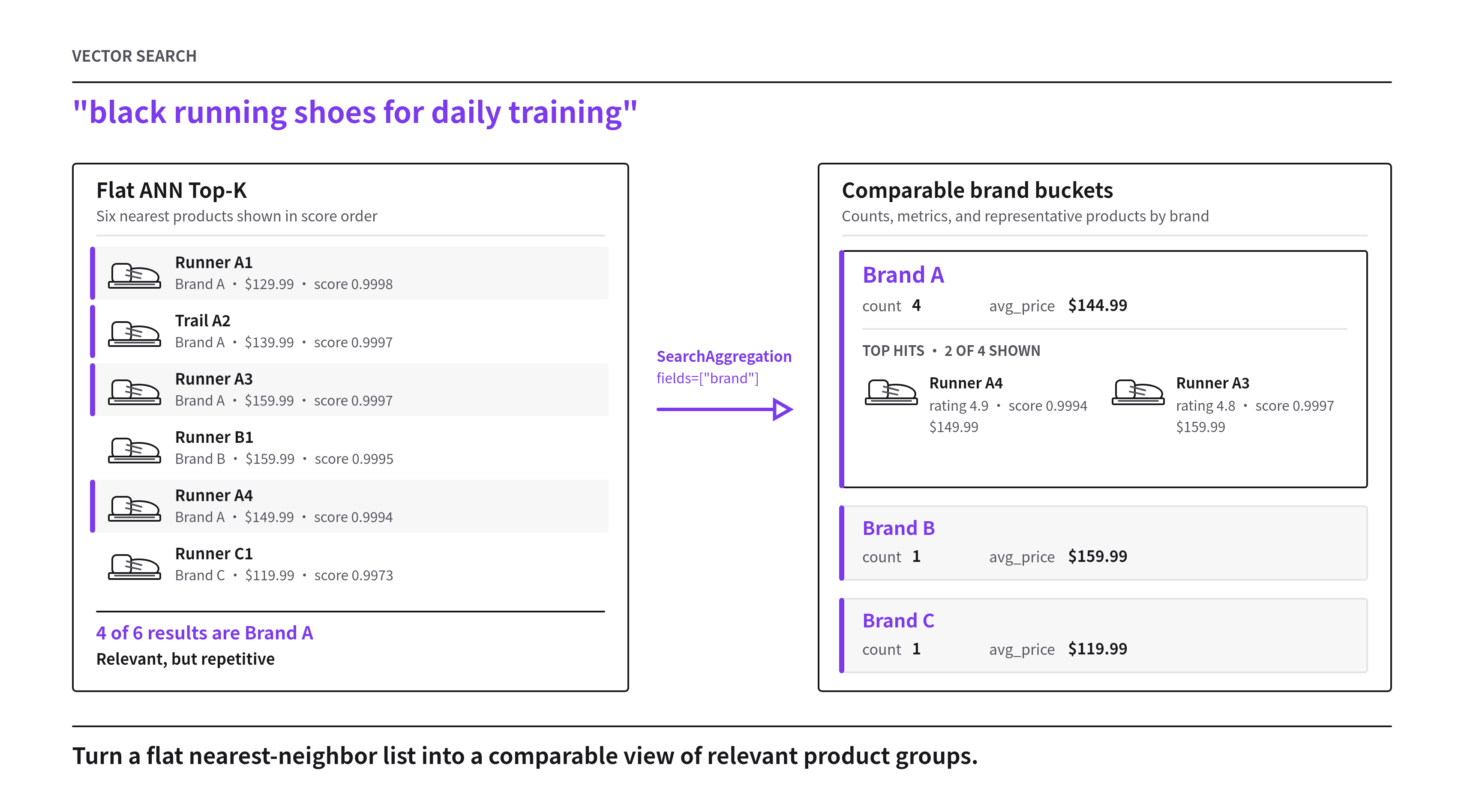 A flat running-shoe search result becomes a set of comparable brand buckets
Search Aggregation does not run an exact full-collection aggregation. Bucket existence, counts, metrics, ordering, and representative hits depend on the candidates retained by the ANN and grouping stages.
How it works
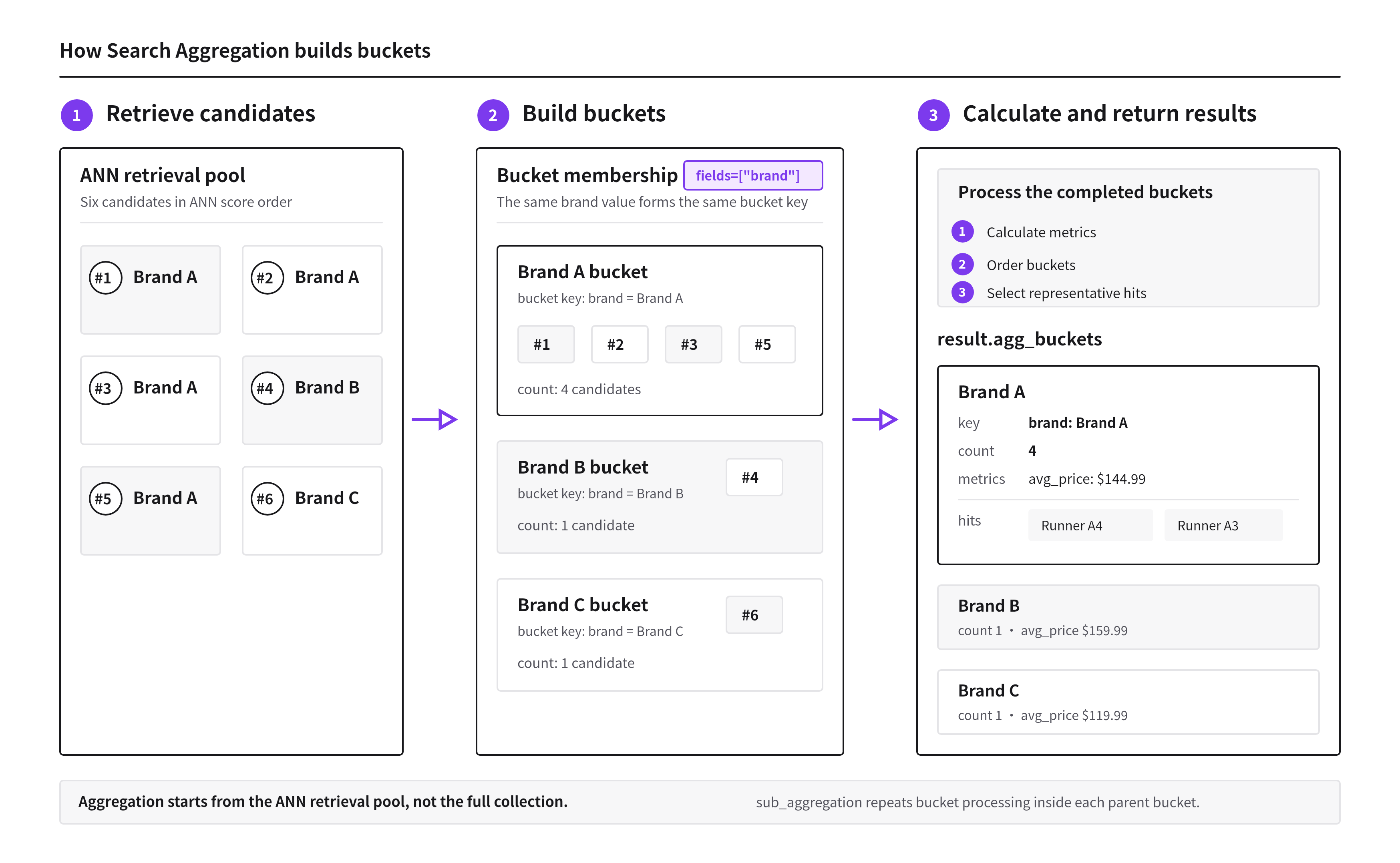 ANN candidates grouped by bucket keys and returned with counts, metrics, and representative hits
Retrieve candidates. Milvus runs ANN search to find entities closest to the query vector. The grouping stage then retains a bounded number of candidates for each full composite key. This per-key candidate budget is the largest
TopHits.sizeanywhere in the aggregation tree, or1when no level configurestop_hits.Build buckets.
SearchAggregation.fieldsdefines the bucket key. Each unique combination of field values creates a separate key. In the figure,fields=["brand"]creates(Brand A),(Brand B), and(Brand C)bucket keys. Retained candidates with the same key belong to the same bucket and contribute to itscount.SearchAggregation.sizelimits how many buckets Milvus returns.Calculate and return results. Each returned bucket contains its key and retained-candidate count. Milvus can also calculate configured metrics, order the buckets, return representative entities, and build child buckets. Each
AggregationBucketinresult.agg_bucketsexposeskey,count,metrics,hits, andsub_groups. When Search Aggregation is enabled, the ordinary search-hit list is empty.
In the diagram, TopHits.size=4 supplies a per-key candidate budget of four, so the four retained Brand A candidates produce count: 4. The completed Brand A card shows only two of the four returned representative hits to keep the figure compact.
With sub_aggregation, Milvus repeats steps 2 and 3 inside each parent bucket. Changes in ANN recall or the per-key candidate budget can change bucket counts, metrics, ordering, hits, and nested results.
Limits
Before using Search Aggregation, note the following limits:
Nested aggregations: A request can contain one root
SearchAggregationand up to three nestedsub_aggregationlevels, for a maximum of four levels in total. Across all levels, at most 10 fields can be used to create bucket keys.Fields used to create bucket keys:
SearchAggregation.fieldssupports Boolean, integer,VARCHAR, andTIMESTAMPTZfields. It does not supportFLOAT,DOUBLE,ARRAY,JSON,GEOMETRY,TEXT, vector, or dynamic fields.Metric fields:
countaccepts"*"or any non-JSON, non-dynamic field and skipsNULLvalues when a field is specified.sumandavgaccept integer and floating-point fields.minandmaxadditionally accept string andTIMESTAMPTZfields.Top Hits sorting fields:
TopHits.sortaccepts comparable Boolean, integer, floating-point, string, andTIMESTAMPTZfields, plus_score. It does not supportARRAY,JSON,GEOMETRY, vector, or dynamic fields.Candidate budget: The largest
TopHits.sizeanywhere in the aggregation tree is also the number of candidates retained per full composite key. If no level configurestop_hits, Milvus retains one candidate per key. Bucketcountand metrics are calculated from these retained candidates, so changingTopHits.sizecan change them.Nullable bucket fields: A
NULLvalue forms its own bucket key. To exclude the null bucket, add a filter such asbrand is not nullto the search request.Repeated fields: The same field cannot appear in more than one
SearchAggregation.fieldslist. For example, if the root aggregation usesfields=["category"], a nestedsub_aggregationcannot also usefields=["category"].Unsupported combinations: Search Aggregation cannot be combined with a non-zero
offset, Search Iterators, Hybrid Search, a Highlighter, or Grouping Search. A top-leveloffsetvalue of0is equivalent to omitting the parameter. In REST v2 search requests,searchAggregationandidscannot be specified together.Returned entries: By default, Milvus rejects a Search Aggregation request when the request’s calculated maximum number of result entries exceeds 10,000. This threshold is controlled by
proxy.maxSearchAggregationResultEntries. Set the configuration value to0or a negative number to disable this check.Milvus calculates this maximum as:
number of query vectors × product of the effective search_size at every aggregation level × largest TopHits.size at any levelFor this server-side calculation, the effective
search_sizeat a level is the explicitly configuredsearch_size, or that level’ssizewhensearch_sizeis omitted. The PyMilvus API used in this guide does not currently exposesearch_size, so PyMilvus requests use each level’ssizefor this calculation. Use1for the last factor when no level configuresTopHits. For example, one query vector, 10 root buckets, five child buckets per root bucket, and two hits per child bucket produce a calculated maximum of:1 × 10 × 5 × 2 = 100
Use Search Aggregation
Choose an example based on what you want to accomplish:
| Go to | Description | Key settings |
|---|---|---|
| Compare and sort buckets | Calculate per-bucket statistics to compare buckets, then sort the returned buckets by metrics, counts, or keys. | fields, size, metrics, order |
| Show representative results from each bucket | Return a limited number of entities from each bucket and sort those entities independently by scalar fields or vector score. | top_hits, TopHits.size, TopHits.sort |
| Group results at multiple levels | Organize results into parent and child bucket levels to analyze multiple dimensions in sequence. | sub_aggregation |
The examples below use a product collection with brand, category, color, price, and rating fields. All brand names, product names, prices, ratings, and search results are synthetic example data. Expand the following section to create the collection and define the shared search variables.
from pymilvus import DataType, MilvusClient, SearchAggregation, TopHits

client = MilvusClient(
    uri="http://localhost:19530",
    token="root:Milvus",
)

collection_name = "product_search_aggregation"

if client.has_collection(collection_name):
    client.drop_collection(collection_name)

schema = client.create_schema(auto_id=False, enable_dynamic_field=False)
schema.add_field("id", DataType.INT64, is_primary=True)
schema.add_field("embedding", DataType.FLOAT_VECTOR, dim=5)
schema.add_field("name", DataType.VARCHAR, max_length=200)
schema.add_field("brand", DataType.VARCHAR, max_length=100)
schema.add_field("category", DataType.VARCHAR, max_length=100)
schema.add_field("color", DataType.VARCHAR, max_length=50)
schema.add_field("price", DataType.DOUBLE)
schema.add_field("rating", DataType.DOUBLE)
schema.add_field("in_stock", DataType.BOOL)

index_params = client.prepare_index_params()
index_params.add_index(
    field_name="embedding",
    index_type="AUTOINDEX",
    metric_type="COSINE",
)

client.create_collection(
    collection_name=collection_name,
    schema=schema,
    index_params=index_params,
    # Make preceding writes visible to searches from this client.
    consistency_level="Session",
)

client.insert(
    collection_name=collection_name,
    data=[
        {
            "id": 1,
            "embedding": [0.12, 0.42, 0.18, 0.66, 0.31],
            "name": "Runner A1",
            "brand": "Brand A",
            "category": "running_shoes",
            "color": "black",
            "price": 129.99,
            "rating": 4.7,
            "in_stock": True,
        },
        {
            "id": 2,
            "embedding": [0.10, 0.39, 0.20, 0.61, 0.29],
            "name": "Trail A2",
            "brand": "Brand A",
            "category": "running_shoes",
            "color": "blue",
            "price": 139.99,
            "rating": 4.6,
            "in_stock": True,
        },
        {
            "id": 3,
            "embedding": [0.14, 0.44, 0.19, 0.68, 0.33],
            "name": "Runner B1",
            "brand": "Brand B",
            "category": "running_shoes",
            "color": "white",
            "price": 159.99,
            "rating": 4.8,
            "in_stock": True,
        },
        {
            "id": 4,
            "embedding": [0.16, 0.41, 0.22, 0.62, 0.30],
            "name": "Runner C1",
            "brand": "Brand C",
            "category": "running_shoes",
            "color": "red",
            "price": 119.99,
            "rating": 4.4,
            "in_stock": False,
        },
        {
            "id": 5,
            "embedding": [0.48, 0.20, 0.59, 0.15, 0.71],
            "name": "Jacket A1",
            "brand": "Brand A",
            "category": "jackets",
            "color": "black",
            "price": 99.99,
            "rating": 4.5,
            "in_stock": True,
        },
        {
            "id": 6,
            "embedding": [0.45, 0.18, 0.55, 0.17, 0.69],
            "name": "Jacket B1",
            "brand": "Brand B",
            "category": "jackets",
            "color": "blue",
            "price": 89.99,
            "rating": 4.3,
            "in_stock": True,
        },
        {
            "id": 7,
            "embedding": [0.09, 0.38, 0.17, 0.60, 0.27],
            "name": "Runner A3",
            "brand": "Brand A",
            "category": "running_shoes",
            "color": "black",
            "price": 159.99,
            "rating": 4.8,
            "in_stock": True,
        },
        {
            "id": 8,
            "embedding": [0.13, 0.43, 0.21, 0.65, 0.32],
            "name": "Runner A4",
            "brand": "Brand A",
            "category": "running_shoes",
            "color": "black",
            "price": 149.99,
            "rating": 4.9,
            "in_stock": True,
        },
    ],
)

client.load_collection(collection_name)

query_vector = [0.11, 0.40, 0.19, 0.64, 0.30]
search_params = {
    "metric_type": "COSINE",
    "params": {},
}
The setup above configures COSINE for both the vector index and the search parameters. Therefore, later examples use {"_score": "desc"} to place higher cosine similarity first. For a distance metric such as L2, use {"_score": "asc"}.
Compare and sort buckets
Use this pattern when you need to compare groups of retrieved entities using calculated statistics and control the order in which the buckets are returned. In this example, Milvus groups retrieved products by brand, calculates price metrics for each brand bucket, and sorts the buckets by average price.
If your goal is only to improve result diversity by returning one or more entities per field value, use Grouping Search instead.
The following configuration creates up to three brand buckets, calculates metrics for each bucket, and sorts the buckets by average price:
aggregation = SearchAggregation(
    # Form one bucket for each distinct brand value.
    fields=["brand"],
    # Return up to three buckets at this aggregation level.
    size=3,
    # Calculate named metrics for every selected bucket.
    metrics={
        "product_count": {"count": "*"},
        "avg_price": {"avg": "price"},
        "min_price": {"min": "price"},
    },
    # Sort buckets by average price, highest first.
    order=[
        {"avg_price": "desc"},
        # If average prices are equal, sort by bucket key in ascending order.
        {"_key": "asc"},
    ],
)
Pass the object to the search_aggregation parameter of MilvusClient.search():
result = client.search(
    collection_name=collection_name,
    data=[query_vector],
    anns_field="embedding",
    search_params=search_params,
    output_fields=[
        "name",
        "brand",
        "category",
        "color",
        "price",
        "rating",
        "in_stock",
    ],
    search_aggregation=aggregation,
)
When search_aggregation is set, PyMilvus returns no ordinary entity hits in result[0]. Read the bucket response from result.agg_buckets[0] instead. The output_fields parameter controls which scalar fields appear in each returned AggregationHit.fields mapping; Milvus can still use metric-source and sort fields that are not listed in output_fields.
The following output was captured from the request above and serialized as JSON for readability. PyMilvus returns AggregationBucket objects rather than JSON. The key value is always an ordered list of key components, even when fields contains only one field. This preserves field order for composite keys.
[
  {
    "key": [
      {
        "field_id": 103,
        "field_name": "brand",
        "value": "Brand B"
      }
    ],
    "count": 1,
    "metrics": {
      "product_count": 1,
      "avg_price": 159.99,
      "min_price": 159.99
    },
    "hits": [],
    "sub_groups": []
  },
  {
    "key": [
      {
        "field_id": 103,
        "field_name": "brand",
        "value": "Brand A"
      }
    ],
    "count": 1,
    "metrics": {
      "product_count": 1,
      "avg_price": 129.99,
      "min_price": 129.99
    },
    "hits": [],
    "sub_groups": []
  },
  {
    "key": [
      {
        "field_id": 103,
        "field_name": "brand",
        "value": "Brand C"
      }
    ],
    "count": 1,
    "metrics": {
      "product_count": 1,
      "avg_price": 119.99,
      "min_price": 119.99
    },
    "hits": [],
    "sub_groups": []
  }
]
For the single query vector in this guide, read the returned top-level buckets from result.agg_buckets[0]. Each bucket exposes its ordered key components, retained-candidate count, calculated metrics, representative hits, and nested buckets in sub_groups.
Read the configuration as follows:
| Setting | What it controls | In this example |
|---|---|---|
fields | How Milvus creates bucket keys | Creates one bucket for each distinct brand value. |
size | The maximum number of returned buckets | Returns up to three brand buckets. |
metrics | The statistics calculated for each bucket | Calculates product count, average price, and minimum price. |
order | How Milvus sorts the returned buckets | Sorts by average price, then uses the bucket key to break ties. |
Milvus ignores limit when search_aggregation is set. Use the root SearchAggregation.size value to control the number of top-level buckets.
With these settings, Milvus returns the Brand B, Brand A, and Brand C buckets in descending avg_price order. The _key criterion applies only when buckets have the same average price. Because this configuration does not define top_hits, every bucket’s hits list is empty and the per-key candidate budget is 1. The displayed counts and metrics therefore describe one retained candidate per brand. Configure top_hits with a larger TopHits.size when the aggregation needs a wider per-key metric window.
Each SearchAggregation.metrics entry maps a user-defined alias to {operation: source}:
| Source | Supported operations | Behavior |
|---|---|---|
Any non-JSON, non-dynamic field | count | Counts retained candidates whose source field is not NULL. |
| Integer or floating-point field | sum, avg, min, max | Calculates over non-null retained values. |
String or TIMESTAMPTZ field | min, max | Selects the minimum or maximum non-null retained value. |
"*" | count | Counts every retained candidate in the bucket. The result matches bucket.count. |
_score | sum, avg, min, max | Aggregates ANN similarity or distance values for retained candidates. |
SearchAggregation.order accepts the following keys:
| Order key | Meaning |
|---|---|
| A metric alias | Sorts by a value calculated in metrics at the same aggregation level, such as avg_price. |
_count | Sorts by the number of retained candidates in each bucket. |
_key | Sorts by the bucket key rather than a collection field named _key. |
Each order entry maps a key to "asc" or "desc". Milvus evaluates multiple entries from first to last. If you omit order, Milvus keeps the bucket discovery order from the retained candidate set.
To sort buckets by vector match quality, first calculate a bucket-level metric from _score, and then use the metric alias in order. You cannot use _score directly as a bucket-order key because each bucket can contain multiple entity scores. For example, with COSINE or IP:
aggregation = SearchAggregation(
    fields=["brand"],
    size=3,
    metrics={"max_score": {"max": "_score"}},
    order=[{"max_score": "desc"}],
)
With L2, calculate the minimum _score value and sort the metric alias in ascending order so that buckets with the lowest distance come first.
To create a composite bucket key, pass multiple field names in the same list:
aggregation = SearchAggregation(
    # Combine brand and color to form a composite bucket key.
    fields=["brand", "color"],
    size=6,
)
This configuration can produce keys such as (Brand A, black), (Brand A, blue), and (Brand B, white). Two entities share a bucket only when both values match. Milvus preserves the list order, so brand is the first key component and color is the second. When _key is used in order, Milvus compares composite key components in the same order. Pass multiple strings in one flat list; nested lists are not supported.
size=6 is the maximum number of composite buckets returned at this aggregation level. The example data contains five distinct brand-color combinations, so all five can be returned. In the returned-entry limit, this request contributes 1 query vector × 6 buckets × 1 = 6 configured result entries.
Multiple fields in one SearchAggregation.fields list create a composite bucket key at that aggregation level. To create a parent-child bucket hierarchy, use a nested aggregation.
The examples that follow redefine aggregation. Pass the updated object to the same search_aggregation parameter and rerun the search call.
Show representative results from each bucket
Include representative entities when the application needs to show actual products from each bucket. In this example, Milvus returns up to two products from each brand bucket, ordered by rating and then by vector score.
Configure TopHits as follows:
aggregation = SearchAggregation(
    fields=["brand"],
    size=3,
    # Return and sort representative entities for each selected bucket.
    top_hits=TopHits(
        # Return up to two entities per bucket.
        size=2,
        # Apply sort criteria in list order.
        sort=[
            {"rating": "desc"},
            {"_score": "desc"},
        ],
    ),
)
The following Brand A bucket was captured from the request above and serialized as JSON for readability.
{
  "key": [
    {
      "field_id": 103,
      "field_name": "brand",
      "value": "Brand A"
    }
  ],
  "count": 2,
  "metrics": {},
  "hits": [
    {
      "pk": 1,
      "score": 0.99976646900177,
      "fields": {
        "brand": "Brand A",
        "category": "running_shoes",
        "color": "black",
        "in_stock": true,
        "name": "Runner A1",
        "price": 129.99,
        "rating": 4.7
      }
    },
    {
      "pk": 2,
      "score": 0.9997048377990723,
      "fields": {
        "brand": "Brand A",
        "category": "running_shoes",
        "color": "blue",
        "in_stock": true,
        "name": "Trail A2",
        "price": 139.99,
        "rating": 4.6
      }
    }
  ],
  "sub_groups": []
}
| Parameter | Purpose |
|---|---|
top_hits | Optional. Configures representative entities for this aggregation level. If omitted, bucket.hits is empty and the per-key candidate budget defaults to one. |
TopHits.size | Returns up to two representative entities from each selected bucket and sets the per-key candidate budget to two for the entire aggregation tree. |
TopHits.sort | Orders entities inside each bucket using the listed criteria. |
Configure top_hits when the application needs representative entities or when counts and metrics need a wider per-key candidate window. A larger TopHits.size increases both the candidate budget and the maximum returned-entry calculation in Limits.
SearchAggregation.order sorts buckets, while TopHits.sort sorts the retained entities inside each bucket. The sort order does not change which candidates were retained for count and metrics. TopHits.sort accepts supported comparable scalar field names and the built-in _score field, which represents the ANN similarity or distance. Milvus evaluates the sort entries from first to last. In this example, it orders products by rating from highest to lowest and uses _score only when two ratings are equal. Because the setup uses COSINE, descending _score places the more similar product first.
The fields used by metrics or TopHits.sort do not have to appear in output_fields. Milvus fetches those fields internally, but only fields explicitly listed in output_fields are included in each returned hit’s fields mapping. Primary keys and vector scores remain available through AggregationHit.pk and AggregationHit.score.
Each returned AggregationHit exposes its primary key in pk, vector score in score, and requested output fields in fields.
Group results at multiple levels
Use nested aggregation when you need one level of buckets inside another. In this example, Milvus creates category buckets first, and then creates brand buckets within each category.
The child aggregation receives only the entities assigned to its parent bucket. fields controls the bucket key at each aggregation level, while sub_aggregation creates the parent-child hierarchy.
The configuration below creates a category bucket with the key (running_shoes). Within that parent bucket, the child aggregation creates separate brand buckets with keys such as (Brand A), (Brand B), and (Brand C).
Parent bucket key:
(running_shoes)

Child bucket keys:
├── (Brand A)
├── (Brand B)
└── (Brand C)
Each level can independently use multiple fields. For example, using fields=["brand", "color"] in the child aggregation would create composite child keys such as (Brand A, black).
The following configuration implements this hierarchy:
aggregation = SearchAggregation(
    fields=["category"],
    size=2,
    metrics={
        "product_count": {"count": "*"},
        "avg_price": {"avg": "price"},
    },
    order=[{"product_count": "desc"}],
    # For each category bucket, group only its entities by brand.
    sub_aggregation=SearchAggregation(
        fields=["brand"],
        size=3,
        metrics={
            "brand_count": {"count": "*"},
            "avg_rating": {"avg": "rating"},
        },
        order=[{"avg_rating": "desc"}],
        top_hits=TopHits(
            size=2,
            sort=[{"rating": "desc"}],
        ),
    ),
)
The following serialized excerpt shows the running_shoes parent bucket and its Brand B child bucket. The Brand A and Brand C child buckets are omitted for brevity.
{
  "key": [
    {
      "field_id": 104,
      "field_name": "category",
      "value": "running_shoes"
    }
  ],
  "count": 4,
  "metrics": {
    "avg_price": 137.49,
    "product_count": 4
  },
  "hits": [],
  "sub_groups": [
    {
      "key": [
        {
          "field_id": 103,
          "field_name": "brand",
          "value": "Brand B"
        }
      ],
      "count": 1,
      "metrics": {
        "avg_rating": 4.8,
        "brand_count": 1
      },
      "hits": [
        {
          "pk": 3,
          "score": 0.9994542598724365,
          "fields": {
            "brand": "Brand B",
            "category": "running_shoes",
            "color": "white",
            "in_stock": true,
            "name": "Runner B1",
            "price": 159.99,
            "rating": 4.8
          }
        }
      ],
      "sub_groups": []
    }
  ]
}
The displayed result represents the bucket path (running_shoes) → (Brand B), not a single composite bucket key (running_shoes, Brand B).
Milvus first selects up to two category buckets, ordered by product_count. It then runs sub_aggregation independently within each selected category and returns up to three brand buckets, ordered by avg_rating.
In the output above:
- The root
running_shoesbucket contains four retained candidates across its child composite keys. Itsmetricscontain the root-levelavg_priceandproduct_countvalues. - The root bucket’s
sub_groupslist contains the child brand buckets. The displayed Brand B bucket contains one retained candidate and its ownavg_ratingandbrand_countvalues. - The root bucket’s
hitslist is empty because the root aggregation does not configuretop_hits. The Brand B child contains a representative hit becausetop_hitsis configured insub_aggregation.
FAQ
How accurate are bucket counts and metrics?
Search Aggregation summarizes retained ANN candidates. It does not run a full-collection aggregation.
Candidate retention has two approximation stages. ANN search can omit relevant collection entities, and the grouping stage retains at most the largest TopHits.size candidates for each full composite key. If no level configures top_hits, this per-key limit is one.
For example, suppose a collection contains 5,000 Brand A products and many are relevant to the vector query. If the aggregation uses TopHits(size=4), the Brand A bucket can retain at most four candidates for a full composite key. Its count and metrics describe those retained candidates, not all relevant Brand A products and not all 5,000 collection entities.
Approximation matters most when order uses a metric alias. Changes in search recall can change the metric values and therefore change which buckets fit within SearchAggregation.size. Nested aggregation can amplify this effect because each child level operates on the entities available in its parent bucket.
If you need exact statistics over every matching entity, use an exact query aggregation workflow instead of Search Aggregation.
How does Search Aggregation differ from Grouping Search?
Choose based on the application’s primary result shape:
| Primary need | Prefer | Response to consume |
|---|---|---|
| Return a standard ranked entity list with fewer repeated values in a grouping field | Grouping Search | Flat search hits for each query vector |
| Inspect or compare groups as buckets, with keys, counts, metrics, ordering, representative hits, or child buckets | Search Aggregation | AggregationBucket objects in result.agg_buckets |
Even when Search Aggregation configures top_hits, its primary response remains a bucket tree. Grouping Search remains useful when the application already processes ordinary search hits and primarily wants result diversity.
The APIs are mutually exclusive. PyMilvus raises ParamError when search_aggregation is combined with group_by_field or group_by_fields in the same request.