How to Use Hybrid Spatial and Vector Search with Milvus

A query like “find romantic restaurants within 3 km” sounds simple. It’s not, because it combines location filtering and semantic search. Most systems need to split this query across two databases, which means syncing data, merging results in code, and extra latency.

Milvus 2.6.4 eliminates this split. With a native GEOMETRY data type and an R-Tree index, Milvus can apply location and semantic constraints together in a single query. This makes hybrid spatial and semantic search much easier and more efficient.

This article explains why this change was needed, how GEOMETRY and R-Tree work inside Milvus, what performance gains to expect, and how to set it up with the Python SDK.

The Limitations of Traditional Geo and Semantic Search

Queries like “romantic restaurants within 3 km” are hard to handle for two reasons:

• “Romantic” needs semantic search. The system has to vectorize restaurant reviews and tags, then find matches by similarity in embedding space. This only works in a vector database.
• “Within 3 km” needs spatial filtering. Results must be restricted to “within 3 km of the user,” or sometimes “inside a specific delivery polygon or administrative boundary.”

In a traditional architecture, meeting both needs usually meant running two systems side by side:

• PostGIS / Elasticsearch for geofencing, distance calculations, and spatial filtering.
• A vector database for approximate nearest neighbor (ANN) search over embeddings.

This “two-database” design creates three practical problems:

• Painful data synchronization. If a restaurant changes its address, you must update both the geo system and the vector database. Missing one update produces inconsistent results.
• Higher latency. The application has to call two systems and merge their outputs, adding network round-trips and processing time.
• Inefficient filtering. If the system ran vector search first, it often returned many results that were far from the user and had to be discarded later. If it applied location filtering first, the remaining set was still large, so the vector search step was still expensive.

Milvus 2.6.4 solves this by adding spatial geometry support directly to the vector database. Semantic search and location filtering now run in the same query. With everything in one system, hybrid search is faster and easier to manage.

What GEOMETRY Adds to Milvus

Milvus 2.6 introduces a scalar field type called DataType.GEOMETRY. Instead of storing locations as separate longitude and latitude numbers, Milvus now stores geometric objects: points, lines, and polygons. Queries like “is this point inside a region?” or “is it within X meters?” become native operations. There’s no need to build workarounds over raw coordinates.

The implementation follows the OpenGIS Simple Features Access standard, so it works with most existing geospatial tooling. Geometry data is stored and queried using WKT (Well-Known Text), a standard text format that is readable by humans and parseable by programs.

Supported geometry types:

• POINT: a single location, such as a store address or a vehicle’s real-time position
• LINESTRING: a line, such as a road centerline or a movement path
• POLYGON: an area, such as an administrative boundary or a geofence
• Collection types: MULTIPOINT, MULTILINESTRING, MULTIPOLYGON, and GEOMETRYCOLLECTION

It also supports standard spatial operators, including:

• Spatial relationships: containment (ST_CONTAINS, ST_WITHIN), intersection (ST_INTERSECTS, ST_CROSSES), and contact (ST_TOUCHES)
• Distance operations: computing distances between geometries (ST_DISTANCE) and filtering objects within a given distance (ST_DWITHIN)

How R-Tree Indexing Works Inside Milvus

GEOMETRY support is built into the Milvus query engine, not just exposed as an API feature. ISpatial data is indexed and processed directly inside the engine using the R-Tree (Rectangle Tree) index.

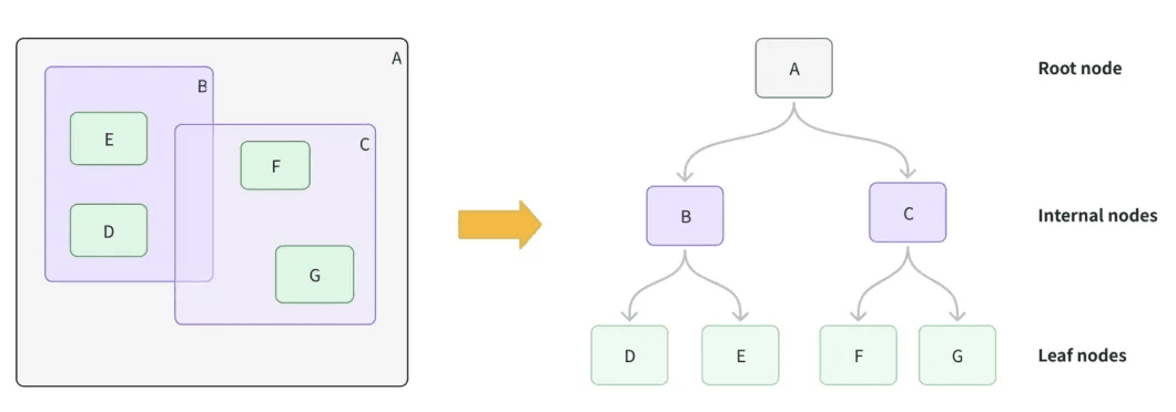
An R-Tree groups nearby objects using minimum bounding rectangles (MBRs). During a query, the engine skips large regions that do not overlap with the query geometry and only runs detailed checks on a small set of candidates. This is much faster than scanning every object.

How Milvus Builds the R-Tree

R-Tree construction happens in layers:

Level	What Milvus Does	Intuitive Analogy
Leaf level	For each geometry object (point, line, or polygon), Milvus computes its minimum bounding rectangle (MBR) and stores it as a leaf node.	Wrapping each item in a transparent box that fits it exactly.
Intermediate levels	Nearby leaf nodes are grouped together (typically 50–100 at a time), and a larger parent MBR is created to cover all of them.	Putting packages from the same neighborhood into a single delivery crate.
Root level	This grouping continues upward until all data is covered by a single root MBR.	Loading all crates onto one long-haul truck.

With this structure in place, spatial query complexity drops from a full scan O(n) to O(log n). In practice, queries over millions of records can go from hundreds of milliseconds down to just a few milliseconds, without losing accuracy.

How Queries are Executed: Two-Phase Filtering

To balance speed and correctness, Milvus uses a two-phase filtering strategy:

• Rough filter: the R-Tree index first checks whether the query’s bounding rectangle overlaps with other bounding rectangles in the index. This quickly removes most unrelated data and keeps only a small set of candidates. Because these rectangles are simple shapes, the check is very fast, but it can include some results that don’t actually match.
• Fine filter: the remaining candidates are then checked using GEOS, the same geometry library used by systems like PostGIS. GEOS runs exact geometry calculations, such as whether shapes intersect or one contains another, to produce correct final results.

Milvus accepts geometry data in WKT (Well-Known Text) format but stores it internally as WKB (Well-Known Binary). WKB is more compact, which cuts storage and improves I/O. GEOMETRY fields also support memory-mapped (mmap) storage, so large spatial datasets don’t need to fit entirely in RAM.

Performance Improvements with R-Tree

Query Latency Stays Flat as Data Grows.

Without an R-Tree index, query time scales linearly with data size — 10x more data means roughly 10x slower queries.

With R-Tree, query time grows logarithmically. On datasets with millions of records, spatial filtering can be tens to hundreds of times faster than a full scan.

Accuracy is Not Sacrificed For Speed

The R-Tree narrows candidates by bounding box, then GEOS checks each one with exact geometry math. Anything that looks like a match but actually falls outside the query area gets removed in the second pass.

Hybrid Search Throughput Improves

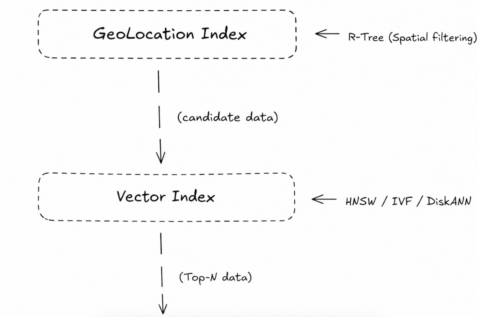
The R-Tree removes records outside the target area first. Milvus then runs vector similarity (L2, IP, or cosine) only on the remaining candidates. Fewer candidates means lower search cost and higher queries per second (QPS).

Getting Started: GEOMETRY with the Python SDK

Define the Collection and Create Indexes

First, define a DataType.GEOMETRY field in the collection schema. This allows Milvus to store and query geometric data.

from pymilvus import MilvusClient, DataType  
import numpy as np  
# Connect to Milvus  
milvus_client = MilvusClient("[http://localhost:19530](http://localhost:19530)")  
collection_name = "lb_service_demo"  
dim = 128  
# 1. Define schema  
schema = milvus_client.create_schema(enable_dynamic_field=True)  
schema.add_field("id", DataType.INT64, is_primary=True)  
schema.add_field("vector", DataType.FLOAT_VECTOR, dim=dim)  
schema.add_field("location", DataType.GEOMETRY)  # Define geometry field  
schema.add_field("poi_name", DataType.VARCHAR, max_length=128)  
# 2. Create index parameters  
index_params = milvus_client.prepare_index_params()  
# Create an index for the vector field (e.g., IVF_FLAT)  
index_params.add_index(  
   field_name="vector",  
   index_type="IVF_FLAT",  
   metric_type="L2",  
   params={"nlist": 128}  
)  
# Create an R-Tree index for the geometry field (key step)  
index_params.add_index(  
   field_name="location",  
   index_type="RTREE"  # Specify the index type as RTREE  
)  
# 3. Create collection  
if milvus_client.has_collection(collection_name):  
   milvus_client.drop_collection(collection_name)  
milvus_client.create_collection(  
   collection_name=collection_name,  
   schema=schema,  
   index_params=index_params,  # Create the collection with indexes attached  
   consistency_level="Strong"  
)  
print(f"Collection {collection_name} created with R-Tree index.")  

Insert Data

When inserting data, geometry values must be in WKT (Well-Known Text) format. Each record includes the geometry, the vector, and other fields.

# Mock data: random POIs in a region of Beijing  
data = []  
# Example WKT: POINT(longitude latitude)  
geo_points = [  
   "POINT(116.4074 39.9042)",  # Near the Forbidden City  
   "POINT(116.4600 39.9140)",  # Near Guomao  
   "POINT(116.3200 39.9900)",  # Near Tsinghua University  
]  
for i, wkt in enumerate(geo_points):  
   vec = np.random.random(dim).tolist()  
   data.append({  
       "id": i,  
       "vector": vec,  
       "location": wkt,  
       "poi_name": f"POI_{i}"  
   })  
res = milvus_client.insert(collection_name=collection_name, data=data)  
print(f"Inserted {res['insert_count']} entities.")  

Run a Hybrid Spatial-Vector Query (Example)

Scenario: find the top 3 POIs that are most similar in vector space and located within 2 kilometers of a given point, such as the user’s location.

Use the ST_DWITHIN operator to apply the distance filter. The distance value is specified in meters.

# Load the collection into memory  
milvus_client.load_collection(collection_name)  
# User location (WKT)  
user_loc_wkt = "POINT(116.4070 39.9040)"  
search_vec = np.random.random(dim).tolist()  
# Build the filter expression: use ST_DWITHIN for a 2000-meter radius filter  
filter_expr = f"ST_DWITHIN(location, '{user_loc_wkt}', 2000)"  
# Execute the search  
search_res = milvus_client.search(  
   collection_name=collection_name,  
   data=[search_vec],  
   filter=filter_expr,  # Inject geometry filter  
   limit=3,  
   output_fields=["poi_name", "location"]  
)  
print("Search Results:")  
for hits in search_res:  
   for hit in hits:  
       print(f"ID: {hit['id']}, Score: {hit['distance']:.4f}, Name: {hit['entity']['poi_name']}")  

Tips for Production Use

• Always create an R-Tree index on GEOMETRY fields. For datasets above 10,000 entities, spatial filters without an RTREE index fall back to a full scan, and performance drops sharply.
• Use a consistent coordinate system. All location data must use the same system (e.g., WGS 84). Mixing coordinate systems breaks distance and containment calculations.
• Pick the right spatial operator for the query. ST_DWITHIN for “within X meters” searches. ST_CONTAINS or ST_WITHIN for geofencing and containment checks.
• NULL geometry values are handled automatically. If the GEOMETRY field is nullable (nullable=True), Milvus skips NULL values during spatial queries. No extra filtering logic needed.

Deployment Requirements

To use these features in production, make sure your environment meets the following requirements.

1. Milvus Version

You must run Milvus 2.6.4 or later. Earlier versions do not support DataType.GEOMETRY or the RTREE index type.

2. SDK Versions

• PyMilvus: upgrade to the latest version (the 2.6.x series is recommended). This is required for proper WKT serialization and for passing RTREE index parameters.
• Java / Go / Node SDKs: check the release notes for each SDK and confirm that they are aligned with the 2.6.4 proto definitions.

3. Built-in Geometry Libraries

The Milvus server already includes Boost.Geometry and GEOS, so you don’t need to install these libraries yourself.

4. Memory Usage and Capacity Planning

R-Tree indexes use extra memory. When planning capacity, remember to budget for geometry indexes as well as vector indexes like HNSW or IVF. The GEOMETRY field supports memory-mapped (mmap) storage, which can reduce memory usage by keeping part of the data on disk.

Conclusion

Location-based semantic search needs more than bolting a geo filter onto a vector query. It requires built-in spatial data types, proper indexes, and a query engine that can handle location and vectors together.

Milvus 2.6.4 solves this with native GEOMETRY fields and R-Tree indexes. Spatial filtering and vector search run in a single query, against a single data store. The R-Tree handles fast spatial pruning while GEOS ensures exact results.

For applications that need location-aware retrieval, this removes the complexity of running and syncing two separate systems.

If you’re working on location-aware or hybrid spatial and vector search, we’d love to hear your experience.

Have questions about Milvus? Join our Slack channel or book a 20-minute Milvus Office Hours session.