Exponential DecayCompatible with Milvus 2.6.x

Exponential decay creates a steep initial drop followed by a long tail in your search results. Like a breaking news cycle where relevance diminishes rapidly at first but some stories retain importance over time, exponential decay applies a sharp penalty to items just beyond your ideal range while still keeping distant items discoverable. This approach is ideal when you want to heavily prioritize proximity or recency but don’t want to completely eliminate more distant options.

Unlike other decay functions:

• Gaussian decay creates a more gradual, bell-shaped decline

• Linear decay decreases at a constant rate until reaching exactly zero

Exponential decay uniquely “frontloads” the penalty, applying most of the relevance reduction early while maintaining a long tail of minimal but non-zero relevance.

When to use exponential decay

Exponential decay is particularly effective for:

Use Case	Example	Why Exponential Works Well
News feeds	Breaking news portals	Quickly reduces relevance of older news while still showing important stories from days ago
Social media timelines	Activity feeds, status updates	Emphasizes fresh content but allows viral older content to surface
Notification systems	Alert prioritization	Creates urgency for recent alerts while maintaining visibility for important ones
Flash sales	Limited-time offers	Rapidly decreases visibility as deadline approaches

Choose exponential decay when:

• Users expect very recent or nearby items to strongly dominate results

• Older or more distant items should still be discoverable if they’re exceptionally relevant

• The relevance drop-off should be front-loaded (steeper at the beginning, more gradual later)

Sharp drop-off principle

Exponential decay creates a curve that drops quickly at first, then gradually flattens into a long tail that approaches but never reaches zero. This mathematical pattern appears frequently in natural phenomena like radioactive decay, population decline, and information relevance over time.

Exp Decay

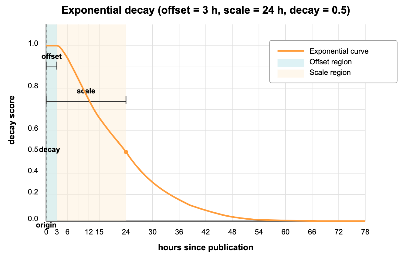
The graph above shows how exponential decay would affect news article rankings in a digital news platform:

• origin (current time): The present moment, where relevance is at its maximum (1.0).

• offset (3 hours): The "breaking news window"—all stories published within the last 3 hours maintain full relevance scores (1.0), ensuring that very recent news isn’t needlessly penalized for minor time differences.

• decay (0.5): The score at the scale distance—this parameter controls how dramatically scores diminish with time.

• scale (24 hours): The time period at which relevance drops to the decay value—news articles exactly 24 hours old have their relevance scores halved (0.5).

As you can see from the curve, news articles older than 24 hours continue to decrease in relevance but never quite reach zero. Even stories from several days ago retain some minimal relevance, allowing important but older news to still appear in your feed (albeit ranked lower).

This behavior mimics how news relevance typically works—very recent stories strongly dominate, but significant older stories can still break through if they’re exceptionally relevant to the user’s interests.

Formula

The mathematical formula for calculating an exponential decay score is:

$$S(doc) = \exp\left( \lambda \cdot \max\left(0, \left|fieldvalue_{doc} - origin\right| - offset \right) \right)$$

Where:

$$\lambda = \frac{\ln(decay)}{scale}$$

Breaking this down in plain language:

1. Calculate how far the field value is from the origin: $|fieldvalue_{doc} - origin|$.

2. Subtract the offset (if any) but never go below zero: $\max(0, distance - offset)$.

3. Multiply by $\lambda$, which is calculated from your scale and decay parameters.

4. Take the exponent, which gives you a value between 0 and 1: $\exp(\lambda \cdot value)$.

The $\lambda$ calculation converts your scale and decay parameters into the rate parameter for the exponential function. A more negative $\lambda$ creates a steeper initial drop.

Use exponential decay

Exponential decay can be applied to both standard vector search and hybrid search operations in Milvus. Below are the key code snippets for implementing this feature.

Create a decay ranker

After your collection is set up with a numeric field (in this example, publish_time), create an exponential decay ranker:

from pymilvus import Function, FunctionType
import datetime

# Create an exponential decay ranker for news recency
ranker = Function(
    name="news_recency",                  # Function identifier
    input_field_names=["publish_time"],   # Numeric field to use
    function_type=FunctionType.RERANK,    # Function type. Must be RERANK
    params={
        "reranker": "decay",              # Specify decay reranker
        "function": "exp",                # Choose exponential decay
        "origin": int(datetime.datetime.now().timestamp()),  # Current time
        "offset": 3 * 60 * 60,            # 3 hour breaking news window
        "decay": 0.5,                     # Half score at scale distance
        "scale": 24 * 60 * 60             # 24 hours (1 day)
    }
)

Apply to standard vector search

After defining your decay ranker, you can apply it during search operations by passing it to the ranker parameter:

# Apply decay ranker to vector search
result = milvus_client.search(
    collection_name,
    data=["market analysis"],             # Query text
    anns_field="dense",                   # Vector field to search
    limit=10,                             # Number of results
    output_fields=["title", "publish_time"], # Fields to return
    ranker=ranker,                        # Apply the decay ranker
    consistency_level="Strong"
)

Apply to hybrid search

Decay rankers can also be applied to hybrid search operations that combine multiple vector fields:

from pymilvus import AnnSearchRequest

# Define dense vector search request
dense = AnnSearchRequest(
    data=["market analysis"],
    anns_field="dense",
    param={},
    limit=10
)

# Define sparse vector search request
sparse = AnnSearchRequest(
    data=["market analysis"],
    anns_field="sparse_vector",
    param={},
    limit=10
)

# Apply decay ranker to hybrid search
hybrid_results = milvus_client.hybrid_search(
    collection_name,
    [dense, sparse],                      # Multiple search requests
    ranker=ranker,                        # Same decay ranker
    limit=10,
    output_fields=["title", "publish_time"]
)

For more information on hybrid search operations, refer to Multi-Vector Hybrid Search.