

Dense and sparse embeddings are two ways of turning text (or other data) into vectors for retrieval. A dense embedding is a fixed-length vector of a few hundred to a few thousand numbers, almost all of them nonzero, where meaning is spread across learned dimensions. A sparse embedding lives in a very large space, usually one dimension per vocabulary term, but only a small number of positions are nonzero, and each one corresponds to a specific term and its weight. Dense vectors excel at paraphrase and meaning; sparse vectors excel at exact terms, names, and codes; and many production systems use both.
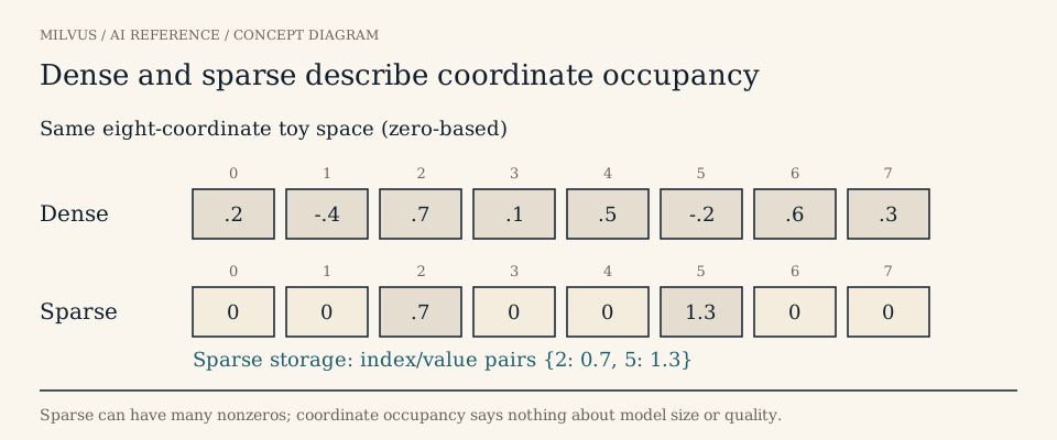 Dense and sparse describe coordinate occupancy, not model size
Dense vs. sparse embeddings at a glance
| Dense embeddings | Sparse embeddings | |
|---|---|---|
| Shape | Fixed dimension, typically 384–3,072 | Vocabulary-sized dimension (tens of thousands to millions), mostly zeros |
| Nonzero values | Nearly all | Usually tens to a few hundred per document |
| What a dimension means | A latent feature with no single readable meaning | A specific token or term |
| Produced by | Neural encoders (sentence transformers, BERT-style bi-encoders, CLIP, commercial embedding APIs) | TF-IDF and BM25 statistics, or learned sparse models such as SPLADE |
| Strong at | Synonyms, paraphrases, conceptual queries, cross-lingual and cross-modal matching | Exact keywords, product codes, error codes, rare names, domain jargon |
| Weak at | Exact identifiers, rare or new terms the model has not seen | Vocabulary mismatch (unless the model expands terms), typos |
| Interpretability | Low | High: you can see which terms contributed to a score |
| Typical index | ANN graph or cluster index (HNSW, IVF, DiskANN) | Inverted index with pruning (WAND, MaxScore) |
| Typical score | Cosine, inner product, or L2 | Inner product or BM25 |
What is a dense embedding?
A dense embedding is the output of a neural encoder that compresses an input into a fixed number of floating-point values. A 768-dimensional sentence embedding is 768 numbers, none of which corresponds to a word. Meaning lives in the pattern across all of them: inputs that the model learned to treat as related end up close together, so “car won’t start” and “engine fails to turn over” can match even though they share no words. The same idea extends beyond text; image, audio, and multimodal models also produce dense vectors in a shared space.
Dense vectors cost a predictable amount of storage: dimension × bytes per value. A 768-dimensional float32 vector takes about 3 KB, so 100 million of them need roughly 300 GB before index overhead, which is why vector quantization matters at scale. Search over dense vectors uses approximate nearest-neighbor indexes because exact comparison against every vector is too slow for large collections.
The main weakness of dense retrieval is precision on literal tokens. An encoder may map ERR_4012 and ERR_4021 to nearly identical vectors, or underweight a rare part number it never saw in training. Dense models also tend to lose quality when moved to a domain far from their training data, a pattern documented in zero-shot benchmarks such as BEIR.
What is a sparse embedding?
A sparse embedding is a vector indexed by vocabulary terms. Picture a vocabulary of 30,000 tokens: the query database error 500 becomes a vector with nonzero weights only at the positions for database, error, and 500, and zeros everywhere else. Because only the nonzero pairs are stored, the vector is compact even though its logical dimension is huge, and you can read it directly to see why a document scored well.
There are two broad families.
Statistical sparse vectors come from term counts and corpus statistics, with no neural network involved. TF-IDF weights a term by how often it appears in a document and how rare it is across the corpus. BM25 refines this with term-frequency saturation (the tenth occurrence of a word adds less than the second) and document-length normalization, controlled by the parameters k1 and b. BM25 remains a strong, robust baseline for keyword-heavy search. See full-text search and BM25.
Learned sparse vectors come from neural models such as SPLADE that predict a weight for each vocabulary term. They keep the interpretable, term-keyed format but can assign weight to related terms that never appeared in the input, a process called term expansion. A query about “laptop battery” might also activate “notebook” and “charge.” That closes part of the vocabulary-mismatch gap that plain BM25 has, while still matching exact tokens well. Some models, such as BGE-M3, output dense and learned sparse vectors from a single forward pass. For a comparison of model families, see dense, sparse, and compact embedding families.
Sparse is not the same as one-hot. A one-hot vector has a single 1; a sparse embedding can have dozens or hundreds of weighted entries. And sparse storage is only cheaper while the nonzero count stays low: an aggressively expanding learned model can produce thousands of nonzeros per document, which can cost more to store and score than a compact dense vector.
How do dense and sparse retrieval differ in practice?
Run three queries against a support knowledge base:
ERR_4012 on login— sparse retrieval finds the article that mentions the exact code; dense retrieval may return generic login-failure articles first.app keeps kicking me out— dense retrieval connects this to articles about session timeouts; BM25 finds little, because the article never uses “kicking” or “out.”session timeout ERR_4012 after password reset— both signals help, and combining them usually ranks best.
This pattern is why the choice is rarely either/or. Dense retrieval wins on meaning, sparse retrieval wins on precision for exact strings, and neither dominates across every query type. The semantic vs. keyword search guide goes deeper on this trade-off.
The two also differ operationally. Dense indexes such as HNSW are built over geometric neighborhoods and tuned with parameters like graph degree and search breadth. Sparse indexes are inverted lists: for each term, the list of documents with a nonzero weight, traversed with algorithms such as WAND or MaxScore that skip documents unable to reach the current top-k. The sparse inverted index guide explains how that differs from dense ANN.
When should you use dense, sparse, or both?
- Dense only fits natural-language questions, conversational search, recommendation, and cross-lingual or image retrieval, where users describe what they mean rather than quote exact text.
- Sparse only fits catalogs, logs, legal or medical text with precise terminology, and any workload where exact identifiers dominate and explainability matters.
- Hybrid (dense + sparse) fits most RAG and enterprise search systems, where queries mix concepts with names, codes, and jargon. Run both retrievals and fuse the result lists, typically with Reciprocal Rank Fusion, which combines ranks rather than raw scores. Fusing raw scores directly is risky because cosine similarity and BM25 live on different scales. See hybrid search.
Keep the extra path only if it improves measured relevance on your own queries. Evaluate dense-only, sparse-only, and fused results on the same labeled set so you can attribute gains to the right signal.
How Milvus stores dense and sparse vectors
Milvus supports both representations as first-class field types, so one collection can hold the text, a dense vector, a sparse vector, and metadata side by side.
- Dense vectors use
FLOAT_VECTOR(orFLOAT16_VECTOR,BFLOAT16_VECTOR,INT8_VECTOR) with a fixeddim, indexed with types such as HNSW, IVF, or DiskANN and scored withCOSINE,IP, orL2. - Sparse vectors use
SPARSE_FLOAT_VECTOR, which needs no declared dimension. You can insert them as a dict ({term_id: weight}), a SciPy sparse matrix, or a list of(index, value)tuples. Indices must lie in the unsigned 32-bit range, values must be non-negative, and each vector needs at least one nonzero entry. They are indexed withSPARSE_INVERTED_INDEX, whereinverted_index_algoselectsDAAT_MAXSCORE(the default),DAAT_WAND, orTAAT_NAIVE.
There are two routes to sparse vectors, and they use different metrics:
- Learned sparse vectors you compute yourself (for example SPLADE or BGE-M3 output) are inserted into a sparse field and searched with
metric_type="IP". - Built-in BM25 full-text search lets Milvus generate the sparse vectors. You define a
VARCHARfield withenable_analyzer=True, attach a BM25Functionthat writes into aSPARSE_FLOAT_VECTORfield, and index that field withmetric_type="BM25"(withbm25_k1andbm25_bas tunable parameters). At query time you pass raw text and Milvus tokenizes and scores it.
from pymilvus import MilvusClient, DataType, Function, FunctionType

schema = MilvusClient.create_schema()
schema.add_field("id", DataType.INT64, is_primary=True, auto_id=True)
schema.add_field("text", DataType.VARCHAR, max_length=4096, enable_analyzer=True)
schema.add_field("dense", DataType.FLOAT_VECTOR, dim=768)
schema.add_field("sparse", DataType.SPARSE_FLOAT_VECTOR)

schema.add_function(Function(
    name="bm25",
    function_type=FunctionType.BM25,
    input_field_names=["text"],
    output_field_names=["sparse"],
))
To combine the two, issue one AnnSearchRequest per vector field and pass them to hybrid_search() with an RRFRanker or WeightedRanker. Milvus returns a single fused list, and you can still apply metadata filters to each request. If quality still falls short, add a reranking stage over the fused candidates.
Related reading
- What are embeddings in vector search?
- What is hybrid search, and when should you use it?
- How does a sparse inverted index differ from dense ANN?
- What is full-text search, and how does BM25 fit?
- How do cosine similarity, inner product, and L2 differ?
Sources and next steps
To try dense, sparse, and hybrid retrieval on the same collection, start with the Milvus Quickstart, then follow the full-text search and hybrid search guides below.


