DiskANN Explained

What is DiskANN?

DiskANN represents a paradigm-shifting approach to vector similarity search. Before that, most vector index types like HNSW rely heavily on RAM to achieve low latency and high recall. While effective for moderate-sized datasets, this approach becomes prohibitively expensive and less scalable as data volumes grow. DiskANN offers a cost-effective alternative by leveraging SSDs to store the index, significantly reducing memory requirements.

DiskANN employs a flat graph structure optimized for disk access, allowing it to handle billion-scale datasets with a fraction of the memory footprint required by in-memory methods. For instance, DiskANN can index up to a billion vectors while achieving 95% search accuracy with 5ms latencies, whereas RAM-based algorithms peak at 100–200 million points for similar performance.

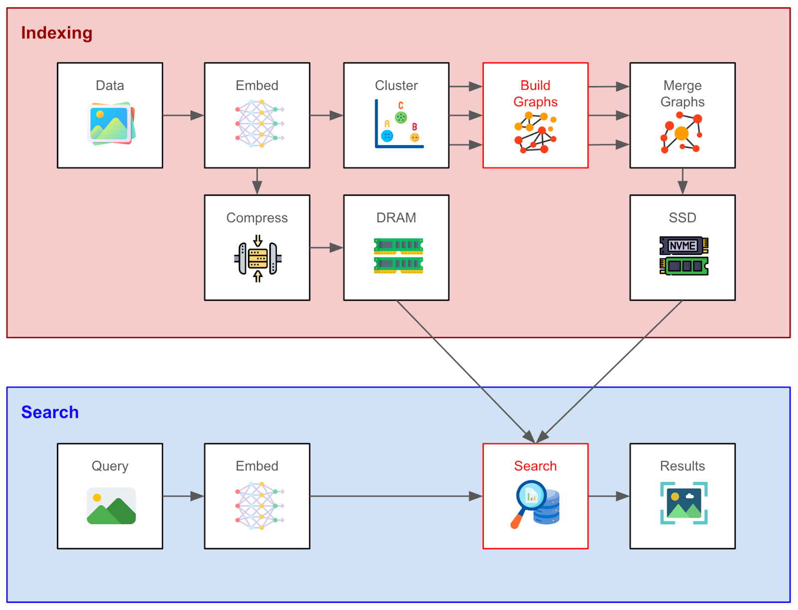
Figure 1: Vector indexing and search workflow with DiskANN

Although DiskANN may introduce slightly higher latency compared to RAM-based approaches, the trade-off is often acceptable given the substantial cost savings and scalability benefits. DiskANN is particularly suitable for applications requiring large-scale vector search on commodity hardware.

This article will explain the clever methods DiskANN has to leverage SSD in addition to RAM and reduce costly SSD reads.

How Does DiskANN Work?

DiskANN is a graph-based vector search method in the same family of methods as HNSW. We first construct a search graph where the nodes correspond to vectors (or groups of vectors), and edges denote that a pair of vectors is “relatively close” in some sense. A typical search randomly chooses an “entry node”, and navigates to its neighbor closest to the query, repeating in a greedy fashion until a local minimum is reached.

Graph-based indexing frameworks differ primarily in how they construct the search graph and perform search. And in this section, we will do a technical deep dive into the innovations of DiskANN for these steps and how they permit low-latency, low-memory performance. (See the above figure for a summary.)

An Overview

We assume that the user has generated a set of document vector embeddings. The first step is to cluster the embeddings. A search graph for each cluster is constructed separately using the Vamana algorithm (explained in the next section), and the results are merged into a single graph. The divide-and-conquer strategy for creating the final search graph significantly reduces memory usage without too greatly affecting search latency or recall.

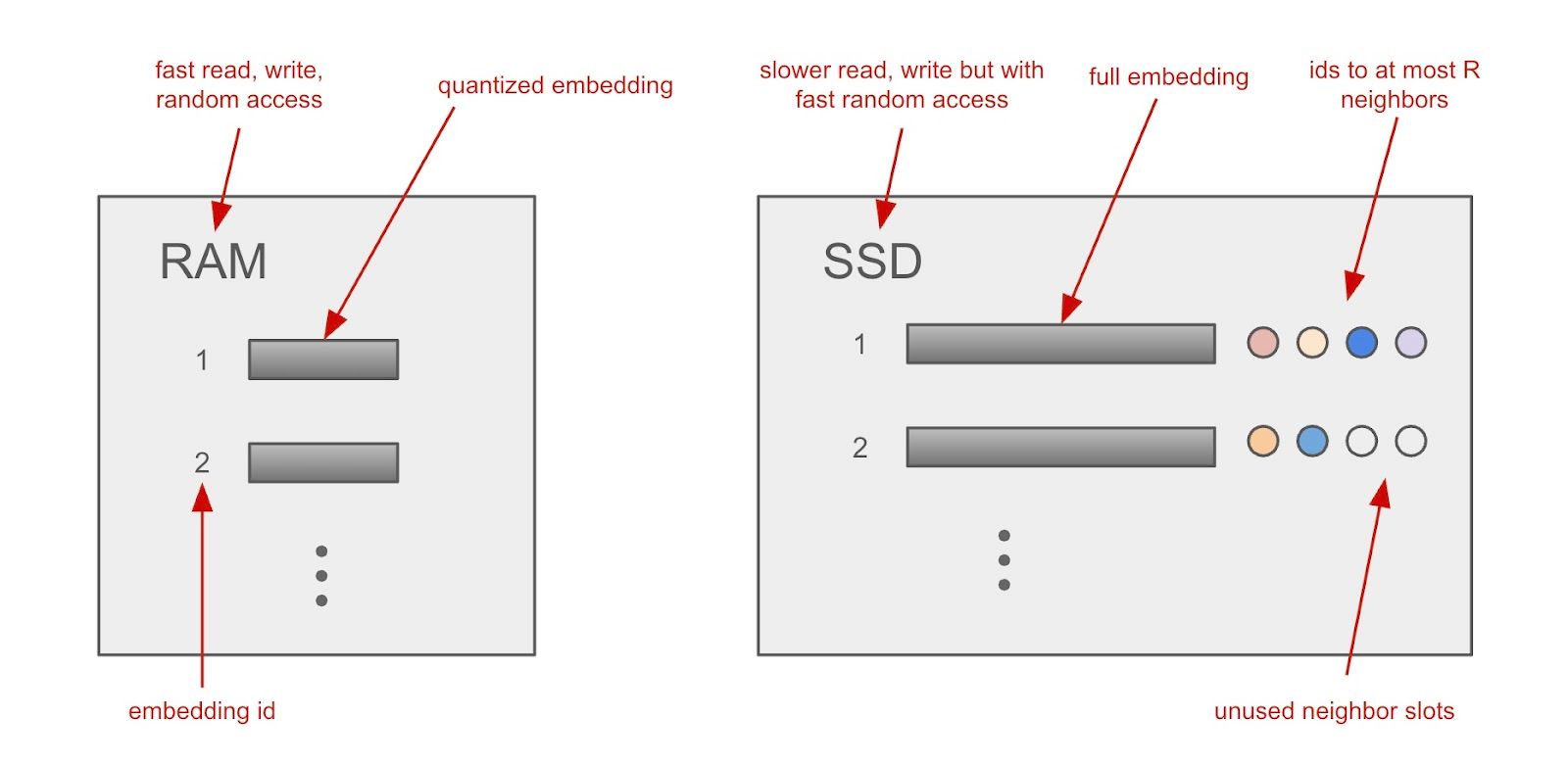
Figure 2: How DiskANN stores vector index across RAM and SSD

Having produced the global search graph, it’s stored on SSD together with the full-precision vector embeddings. A major challenge is to finish the search within a bounded number of SSD reads, since SSD access is expensive relative to RAM access. So, a few clever tricks are used to restrict the number of reads:

First, the Vamana algorithm incentivizes shorter paths between close nodes while capping the maximum number of neighbors of a node. Second, a fixed-size data structure is used to store each node’s embedding and its neighbors (see the above figure). What this means is that we can address a node’s metadata by simply multiplying the data structure size by the node’s index and using this as an offset while simultaneously fetching the node’s embedding. Third, due to how SSD works, we can fetch multiple nodes per read request - in our case, the neighbor nodes - reducing the number of read requests further.

Separately, we compress the embeddings using product quantization and store them in RAM. In doing so, we can fit billions-scale vector datasets into a memory that is feasible on a single machine for quickly calculating approximate vector similarities without disk reads. This provides guidance for reducing the number of neighbor nodes to access next on the SSD. Importantly, however, the search decisions are made using the exact vector similarities, with the full embeddings retrieved from SSD, which ensures higher recall. To emphasize, there is an initial phase of search using quantized embeddings in memory, and a subsequent search on a smaller subset reading from SSD.

In this description, we have glossed over two important albeit involved steps: how to construct the graph, and how to search the graph - the two steps indicated by the red boxes above. Let’s examine each of these in turn.

“Vamana” Graph Construction

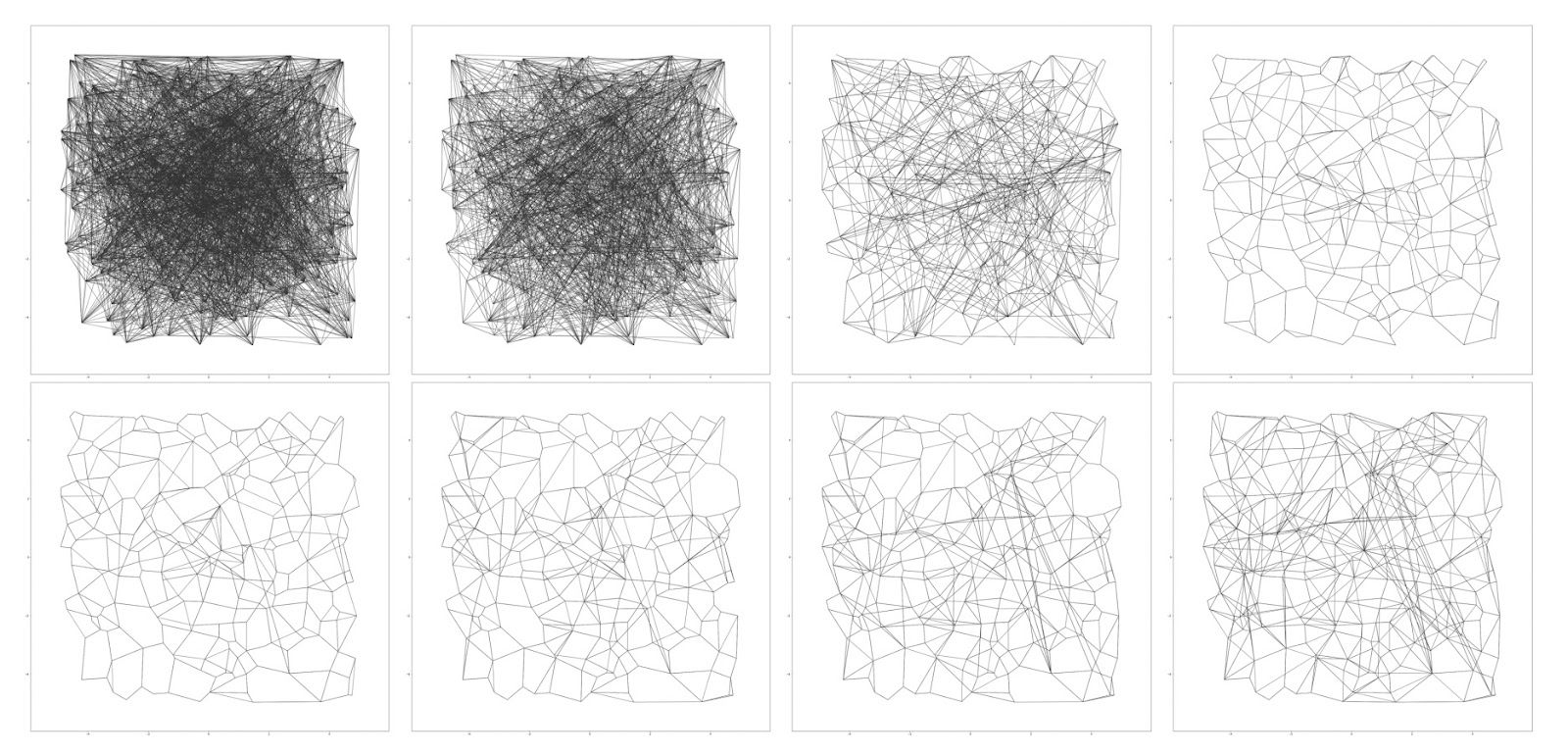
Figure: “Vamana” Graph Construction

The DiskANN authors develop a novel method for constructing the search graph, which they call the Vamana algorithm. It initializes the search graph by randomly adding O(N) edges. This will result in a graph that is “well-connected”, although without any guarantees on greedy search convergence. It then prunes and reconnects the edges in an intelligent way to ensure there are sufficient long-range connections (see above figure). Allow us to elaborate:

Initialization

The search graph is initialized to a random directed graph where each node has R out-neighbors. We also calculate the medoid of the graph, that is, the point that has the minimum average distance to all other points. You can think of this as analogous to a centroid that is a member of the set of nodes.

Search for Candidates

After initialization, we iterate over the nodes, performing both adding and removing edges at each step. First, we run a search algorithm on the selected node, p, to generate a list of candidates. The search algorithm starts at the medoid and greedily navigates closer and closer to the selected node, adding the out-neighbors of the closest node found so far at each step. The list of L found nodes closest to p is returned. (If you’re not familiar with the concept, the medoid of a graph is the point that has the minimum average distance to all other points and acts as an analog of a centroid for graphs.)

Pruning and Adding Edges

The node’s candidate neighbors are sorted by distance, and for each candidate, the algorithm checks whether it is “too close” in direction to an already chosen neighbor. If so, it’s pruned. This promotes angular diversity among neighbors, which empirically leads to better navigation properties. In practice, this means that a search starting from a random node can more quickly reach any target node by exploring a sparse set of long-range and local links.

After pruning edges, edges along the greedy search path to p are added. Two passes of pruning are performed, varying the distance threshold for pruning so that long-term edges are added in the second pass.

What’s Next?

Subsequent work has been built upon DiskANN for additional improvements. One noteworthy example, known as FreshDiskANN, modifies the method to allow for the easy updating of the index after construction. This search index, which provides an excellent tradeoff between performance criteria, is available in the Milvus vector database as the DISKANN index type.

# Prepare index parameters
index_params = client.prepare_index_params()

# Add DiskANN index
index_params.add_index(
    field_name="vector",
    index_type="DISKANN",
    metric_type="COSINE"
)

# Create collection with index
client.create_collection(
    collection_name="diskann_collection",
    schema=schema,
    index_params=index_params
)

You can even tune the DiskANN parameters, such as MaxDegree and BeamWidthRatio: see the documentation page for more details.

Resources

• Milvus Documentation on using DiskANN

• “DiskANN: Fast Accurate Billion-point Nearest Neighbor Search on a Single Node”

• “FreshDiskANN: A Fast and Accurate Graph-Based ANN Index for Streaming Similarity Search”