

HNSW_SQ, HNSW_PQ, and HNSW_PRQ are Milvus index types that keep the HNSW graph but store each vector as a compressed code instead of full float32 values. Scalar quantization (SQ) shrinks every dimension to fewer bits and usually loses very little recall; product quantization (PQ) splits the vector into sub-vectors and replaces each with a codebook ID, which compresses far more aggressively; product residual quantization (PRQ) adds extra residual codebooks on top of PQ to win back accuracy. All three can optionally rerank a shortlist with higher-precision data, which is the main tool for recovering recall.
The short version: start with HNSW_SQ at SQ8 when you need roughly 4x smaller vectors with minimal tuning; move to HNSW_PQ or HNSW_PRQ only when memory is the hard limit and you are prepared to tune m, nbits, and refinement.
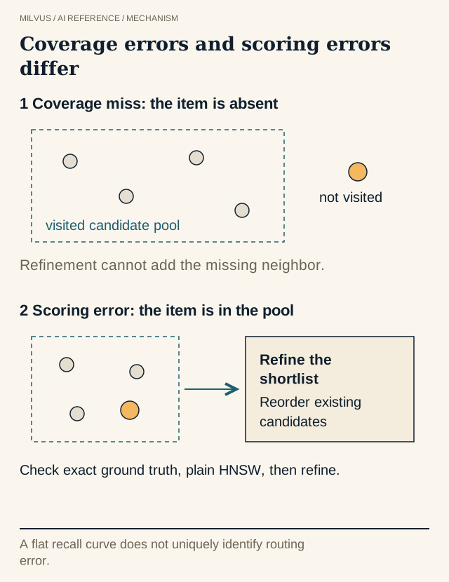 Diagnose a recall plateau step by step. The shape of a recall curve alone does not identify the cause.
Why compress an HNSW index at all?
An HNSW index keeps two things in memory: the vectors and the neighbor links. With modern embeddings the vectors dominate. A 768-dimensional float32 vector takes 3,072 bytes, while its layer-0 links at the default M = 30 take only a few hundred bytes. Compressing the vectors therefore attacks most of the footprint, and it also speeds up each distance calculation because less memory has to be read per hop.
What compression cannot touch is the graph itself. The links are stored the same way in every variant, so the total index never shrinks by the full compression ratio. Keep that in mind when you estimate capacity.
How much smaller does each variant make the vectors?
For a 768-dimensional float32 embedding (3,072 bytes uncompressed), the vector part of the index looks roughly like this:
| Setting | Bytes per vector (codes only) | Approximate ratio |
|---|---|---|
| HNSW (no compression) | 3,072 | 1x |
HNSW_SQ, sq_type="FP16" or "BF16" | 1,536 | 2x |
HNSW_SQ, sq_type="SQ8" | 768 | 4x |
HNSW_SQ, sq_type="SQ6" | 576 | about 5.3x |
HNSW_SQ, sq_type="SQ4U" | 384 | 8x |
HNSW_PQ, m=96, nbits=8 | 96 | 32x |
HNSW_PRQ, m=96, nbits=8, nrq=2 | about 192 | about 16x |
These are code sizes, not total index sizes. Add the graph links, codebooks, and, if you enable refinement, the refinement copy of each vector. The quantization guide explains how each code is formed.
How does each quantizer work inside the graph?
HNSW_SQ maps each dimension to a lower-precision value. SQ8 stores one byte per dimension; SQ6 and SQ4U go lower; FP16 and BF16 keep a 16-bit float. Because every dimension is still represented individually, distances stay close to the originals and the graph navigates almost as well as uncompressed HNSW.
HNSW_PQ divides each vector into m sub-vectors and learns a codebook of 2^nbits centroids for each sub-space. A vector is stored as m centroid IDs, and query distances are computed with lookup tables. This yields the biggest savings, but each distance is now an estimate built from centroids, and the error grows as m or nbits shrinks.
HNSW_PRQ starts with PQ, then quantizes the residual (the difference between the original vector and its PQ approximation) with additional codebooks. nrq sets how many residual passes are applied. More passes capture more detail at the cost of more bytes and a slower build.
Why does compression hurt graph search differently from IVF?
In an IVF index, the candidate set is fixed first by cluster membership, and compression only affects how those candidates are scored. In HNSW, the distances also decide where the search goes next. Each hop moves to the neighbor that looks closest to the query, so if compressed distances are wrong, the walk can turn away from the region that holds the true neighbors. Those neighbors are then never visited, and no amount of reranking can bring them back.
A recall plateau tells you something is limiting the search, but not what. If recall keeps rising as you increase ef, the search is simply under-exploring, and more effort fixes it. If recall flattens well below target, several causes look the same from the outside, so separate them before changing the quantizer:
- Check the measurement. Ground truth must come from an exact search over the same data, metric, normalization, and filter. A mismatch there caps recall no matter what the index does.
- Compare with uncompressed HNSW. Build plain
HNSWwith the sameMandefConstructionon the same data. If it plateaus too, the limit is the graph itself (connectivity,M,efConstruction) or the data, not compression. - Turn on refinement. Enable
refinewith a full-precision or higher-precisionrefine_typeand raiserefine_k. If recall recovers, the true neighbors were being found but mis-scored at the final ranking step, and refinement or a finer quantizer for scoring is the fix. - Only then suspect routing. If plain HNSW reaches target, refinement does not help, and recall still flattens, compressed distances are likely steering the walk away from the true neighbors. A finer quantizer (higher
nbits, largerm, morenrq, or SQ instead of PQ) or a better-connected graph (higherM) are the levers. A sparse graph is less forgiving of per-hop error because it offers fewer alternative paths.
What do refine, refine_type, and refine_k do?
Refinement is a second-stage rerank. When refine=True, Milvus keeps an additional, higher-precision copy of the vectors in the format given by refine_type (SQ6, SQ8, BF16, FP16, or FP32; it must be more precise than the main code). At query time the graph search runs on the compressed codes, then a shortlist is rescored with the refinement data. refine_k is a magnification factor: with limit=10 and refine_k=3, about 30 candidates are rescored and the best 10 returned.
Refinement fixes ranking mistakes among nodes the traversal reached, and it is cheap in latency. Its price is memory: the refinement copy is stored in addition to the codes. Pairing PQ codes with an SQ8 refinement copy is a common middle ground, while FP32 refinement gives back most of the memory you saved.
Milvus parameters at a glance
All three variants share the HNSW graph parameters and the search-time parameters, as documented in the Milvus guides for HNSW_SQ, HNSW_PQ, and HNSW_PRQ:
| Parameter | Applies to | Range | Default |
|---|---|---|---|
M | all | [2, 2048] | 30 |
efConstruction | all | [1, int_max] | 360 |
sq_type | HNSW_SQ | SQ4U, SQ6, SQ8, BF16, FP16 | SQ8 |
m | HNSW_PQ, HNSW_PRQ | [1, 65536]; must divide the vector dimension | none |
nbits | HNSW_PQ, HNSW_PRQ | [1, 24] | 8 |
nrq | HNSW_PRQ | [1, 16] | 2 |
refine | all | true / false | false |
refine_type | all | SQ6, SQ8, BF16, FP16, FP32 | none |
ef (search) | all | [1, int_max] | the search limit |
refine_k (search) | all | [1, float_max) | 1 |
All three support L2, IP, and COSINE. An HNSW_PQ index with refinement looks like this:
index_params = client.prepare_index_params()
index_params.add_index(
    field_name="embedding",
    index_type="HNSW_PQ",
    metric_type="COSINE",
    params={
        "M": 30,
        "efConstruction": 360,
        "m": 96,          # 768 / 96 = 8 dimensions per sub-vector
        "nbits": 8,
        "refine": True,
        "refine_type": "SQ8",
    },
)
client.create_index(collection_name="docs", index_params=index_params)

res = client.search(
    collection_name="docs",
    anns_field="embedding",
    data=[query_vector],
    limit=10,
    search_params={"params": {"ef": 64, "refine_k": 2}},
)
How do you choose between HNSW_SQ, HNSW_PQ, and HNSW_PRQ?
- HNSW_SQ with
SQ8is the low-risk default. Expect small recall loss, a 4x reduction in vector bytes, and no codebook training to tune. - HNSW_SQ with
SQ4UorSQ6squeezes further. Addrefine=Truewithrefine_type="SQ8"or"FP16"if recall drops. - HNSW_PQ is for corpora where even SQ8 does not fit. Choose
mso each sub-vector covers a few dimensions (4 to 8 is a common range) and plan on refinement. - HNSW_PRQ is worth testing when HNSW_PQ is too lossy but you still need well beyond 4x compression. Start at
nrq=2and compare against PQ with a largermat the same byte budget.
If no compressed HNSW variant meets both memory and recall, the bottleneck is probably the in-memory design itself, and DISKANN or an IVF variant may suit you better. The index selection guide puts these options side by side.
How should you benchmark the variants?
Hold the embedding model, data, metric, filters, and queries fixed, and compute exact ground truth with a FLAT index. For each variant, sweep ef (and refine_k if refinement is on) and record Recall@k, p95 latency, throughput, build time, and loaded memory. Compare variants at the same recall, not at the same ef: a smaller index at lower recall is not a like-for-like win. Check the tails as well. Quantizers trained on a skewed sample can do noticeably worse on rare topics, unusual vector norms, or heavily filtered queries, even when the average looks fine. The memory estimation guide helps turn the measured footprint into node counts.
To experiment, create a collection with the Milvus Quickstart and swap index_type between HNSW, HNSW_SQ, HNSW_PQ, and HNSW_PRQ on the same data.


