What is HNSW, and how should you tune it?

HNSW (Hierarchical Navigable Small World) is a graph-based index for approximate nearest-neighbor (ANN) search. It connects every vector to a handful of close neighbors, then stacks progressively sparser copies of that graph on top, so a query can take long hops near the top and short, precise hops at the bottom. The result is search cost that grows roughly logarithmically with collection size, which is why HNSW is the default choice for in-memory, low-latency vector search in most databases, including Milvus.

The method was introduced by Yury Malkov and Dmitry Yashunin (arXiv:1603.09320). Three parameters control almost all of its behavior: M and efConstruction when the graph is built, and ef when it is searched.

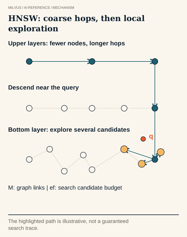HNSW hierarchical graph navigation

How does HNSW work?

HNSW combines two older ideas.

Navigable small-world graphs. If each point links to its nearest neighbors plus a few longer-range links, a greedy walk (“always move to the neighbor closest to the query”) reaches the target region in a small number of hops. A flat graph of this kind works, but on large datasets the walk spends many hops just crossing the space.

Skip lists. A skip list speeds up search in a sorted list by keeping express lanes: higher levels contain fewer elements, so you skip far ahead before dropping down to finer levels. HNSW applies the same trick to a proximity graph.

Building the graph

Vectors are inserted one at a time. Each new vector is assigned a top layer drawn from an exponentially decaying distribution: every vector lives on layer 0, a small fraction also appear on layer 1, a smaller fraction on layer 2, and so on. The normalization constant is usually set to mL = 1/ln(M), which keeps upper layers sparse in a predictable way.

To insert a vector, the algorithm searches greedily from the global entry point down to the new vector’s top layer. From there down to layer 0 it runs a wider search, keeping a candidate list of size efConstruction, and picks up to M neighbors on each layer. A neighbor-selection heuristic prefers neighbors that point in different directions over a tight cluster of near-duplicates, which keeps the graph navigable across cluster boundaries. Layer 0 usually allows about twice as many links (2·M) as the upper layers because it carries the final, fine-grained search.

Searching the graph

1. Start at the entry point on the top layer.
2. Greedily move to whichever neighbor is closer to the query until no neighbor improves the distance (a local minimum on that layer).
3. Drop to the next layer, using that node as the starting point, and repeat.
4. On layer 0, run a best-first search that keeps a dynamic list of the ef closest candidates seen so far, expanding the most promising unvisited node until the list stops improving.
5. Return the top k from that list.

Upper layers act as a coarse map; layer 0 does the precise work. Because the number of layers grows with log N, query cost scales roughly logarithmically with the number of vectors rather than linearly as a brute-force scan does.

What do M, efConstruction, and ef control?

Two points matter in practice. First, ef must be at least k, because the candidate list is where the top k comes from. Second, build parameters set a ceiling: if a graph built with a small M cannot reach your recall target at any ef, raising ef further will not help, and you need to rebuild.

HNSW parameters in Milvus

Milvus exposes HNSW as index_type="HNSW" on float vector fields with the L2, IP, or COSINE metric. According to the Milvus HNSW guide:

Building the index with PyMilvus:

from pymilvus import MilvusClient

client = MilvusClient(uri="http://localhost:19530")

index_params = client.prepare_index_params()
index_params.add_index(
    field_name="embedding",
    index_type="HNSW",
    index_name="embedding_hnsw",
    metric_type="COSINE",
    params={"M": 32, "efConstruction": 200},
)
client.create_index(collection_name="docs", index_params=index_params)

Searching with a per-request ef:

res = client.search(
    collection_name="docs",
    anns_field="embedding",
    data=[query_vector],
    limit=10,
    search_params={"params": {"ef": 64}},
)

Because ef is a search parameter, you can change it per request without rebuilding, for example a lower value for an autocomplete path and a higher value for an offline evaluation job against the same index.

How much memory does HNSW use?

HNSW keeps both the vectors and the graph in memory. A rough per-vector estimate is the raw vector size plus the layer-0 links:

• Vectors: d × 4 bytes for float32. A 768-dimensional embedding is 3,072 bytes.
• Links: about 2·M neighbor IDs on layer 0 at 4 bytes each, plus a small amount for upper layers. With M = 30, that is roughly 240 bytes.

For 10 million 768-d vectors, that works out to about 30 GB of vectors and a few GB of graph. With large embeddings the vectors usually dominate the footprint, which is why compressed variants mostly target the vector side. If memory is the binding constraint, look at HNSW_SQ, HNSW_PQ, and HNSW_PRQ or at disk-based DISKANN before shrinking M. The memory estimation guide walks through a full sizing calculation.

How should you tune HNSW?

A disciplined sequence avoids most wasted rebuilds:

1. Fix the problem first. Choose the embedding model, metric, and dataset, and build an exact ground truth for a few hundred to a few thousand representative queries using a FLAT baseline.
2. Build once with sensible defaults. The Milvus defaults (M=30, efConstruction=360) are a reasonable starting graph. Values of M between about 16 and 64 cover most text and image embeddings.
3. Sweep ef on that graph. Measure Recall@k and p95/p99 latency at several values, for example k, 2k, 4k, and 8k. This gives you the recall/latency curve for that graph.
4. Rebuild only if the curve tops out too low. If recall plateaus below target, increase M (and efConstruction with it). If recall is fine but memory is too high, try a lower M or a quantized variant.
5. Test the real workload. Include metadata filters, concurrency, and the production query mix. Very selective filters change how much of the graph is usable, which is covered in the metadata filtering guide.

Always report latency together with the recall it was measured at. A fast number at 80% recall and a fast number at 98% recall describe different systems.

What are HNSW’s strengths and limits?

Strengths. HNSW delivers high recall at low latency with little tuning, supports incremental insertion without retraining (unlike IVF, which needs k-means centroids), and degrades gracefully as you lower ef.

Limits. It is memory-hungry because both vectors and links must stay resident. Builds are slower than cluster-based indexes, since every insertion runs a search. Deleted vectors cannot simply be removed from a graph without hurting connectivity, so systems mark them deleted and clean up later; in Milvus, deletions are applied at query time and segments are rewritten by compaction, after which indexes are rebuilt. Very restrictive filters can also force the search to visit many nodes before it finds enough matching neighbors.

When should you choose something other than HNSW?

HNSW is the right first candidate when the dataset fits in memory and latency matters. Consider alternatives when capacity or cost dominates: IVF variants for faster builds and quantized storage, DISKANN when the corpus is larger than RAM, or GPU_CAGRA for high-throughput batch search on GPUs. The decision guide on how to choose a vector index compares them side by side, and the ANN overview explains how graph indexes fit among the other families.

To try HNSW end to end, start with the Milvus Quickstart, then set M, efConstruction, and ef using the HNSW reference. If you prefer not to manage index memory yourself, Zilliz Cloud runs managed Milvus.

Related reading

• How do HNSW_SQ, HNSW_PQ, and HNSW_PRQ change the trade-offs?
• How do IVF indexes use centroids to search vectors?
• How should you benchmark vector search performance?
• What is GPU_CAGRA, and when does it help vector search?

Sources

• Malkov and Yashunin, Efficient and robust approximate nearest neighbor search using HNSW graphs
• Milvus HNSW index
• Milvus index structures