

Vector quantization is a lossy compression technique that stores each embedding as a compact code instead of a full array of 32-bit floats, so a vector index needs less memory and can compute approximate distances faster. The cost is precision: distances computed from codes are estimates, so recall can drop unless the system rescans a shortlist with higher-precision vectors. In Milvus, quantization is one layer of an index type such as IVF_SQ8, IVF_PQ, HNSW_SQ, HNSW_PRQ, or IVF_RABITQ.
 Treat compression as another approximation
Quantization is not the same as choosing a smaller embedding model or truncating dimensions. Those change the vector itself. Quantization keeps the dimension count and changes how many bits represent it inside the index.
Why compress vectors at all?
Raw float vectors are expensive. For N vectors of dimension D in FP32, the vector payload alone is N × D × 4 bytes:
| Corpus | Raw FP32 payload |
|---|---|
| 1M × 768 dims | 3.07 GB |
| 100M × 768 dims | 307 GB |
| 100M × 1536 dims | 614 GB |
That is before IDs, scalar fields, graph links, centroids, and allocator overhead. Since most vector indexes are served from memory, the payload directly sets how many machines you need. Compression also speeds search: smaller codes mean more of them fit in CPU cache, and some codes allow distances to be computed with table lookups or bit operations instead of floating-point multiplies. For a fuller accounting of index overhead, see how to estimate memory for vector search.
How does scalar quantization work?
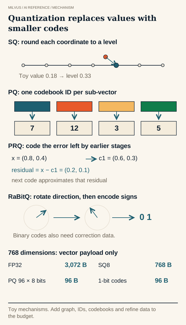
Scalar quantization (SQ) compresses each coordinate independently. The classic 8-bit version finds a value range, normalizes each coordinate into it, and rounds to one of 256 integer levels:
code = round( (x - min) / (max - min) × 255 )
Every dimension shrinks from 4 bytes to 1, so SQ8 cuts the vector payload by 75% (4×). It needs no codebook training beyond the range statistics, it is fast to encode, and the error per coordinate is bounded by the step size. The downside is that 4× is roughly where SQ tops out at good quality; fewer bits per coordinate leave too few levels to represent the value range well.
Lower-precision floats are a gentler variant of the same idea. FP16 and BF16 halve the payload with very little distortion. Milvus’s HNSW_SQ exposes this choice directly through sq_type, which accepts SQ4U, SQ6, SQ8, BF16, and FP16 (default SQ8).
How does product quantization work?
Product quantization (PQ) reaches much higher compression by quantizing groups of dimensions together rather than one coordinate at a time.
- Split. Divide each
D-dimensional vector intomequal subvectors. In Milvus,mmust divide the dimension evenly. - Train codebooks. For each of the
msubspaces, run k-means on a sample of training vectors to learn2^nbitscentroids. With the commonnbits = 8, that is 256 centroids per subspace. - Encode. Replace each subvector with the ID of its nearest centroid. A vector becomes
msmall integers, takingm × nbitsbits.
A worked example: a 768-dimensional vector with m = 96 and nbits = 8 stores a 96-byte code instead of 3,072 bytes, a 32× reduction for the code itself. The shared codebooks add a fixed cost (m × 256 centroids of D/m dimensions each), which is negligible at scale.
Asymmetric distance computation
At query time PQ does not decode vectors. Instead, the query is kept at full precision and split into the same m subvectors. For each subspace the engine precomputes the distance from the query subvector to all 256 centroids, producing an m × 256 lookup table. The approximate distance to any stored vector is then the sum of m table lookups, one per code byte. This is called asymmetric distance computation (ADC) because only the database side is quantized, and it is why PQ search is fast even though the codes are tiny.
PQ quality depends on training. If the sample used to learn codebooks does not resemble production data, or the distribution shifts after re-embedding, the codebooks fit poorly and recall drops. Larger nbits or more subvectors improve accuracy at the price of bigger codes and slower training.
What are residual and binary quantization?
Residual quantization encodes the error that one quantizer leaves behind. After PQ approximates a vector, the residual (original minus approximation) is quantized again, and the codes are combined. Milvus’s HNSW_PRQ does exactly this: PQ with m and nbits, plus nrq residual stages (default 2, range 1–16). More stages tighten the approximation and grow the code.
Binary quantization keeps one bit per dimension, a 32× reduction versus FP32 that lets distances be estimated with XOR/AND and popcount instructions. Naive sign-bit binarization throws away magnitude and often loses too much accuracy for high-recall search. RaBitQ is a more careful binary scheme: it applies a random rotation, normalizes vectors relative to a centroid, and uses an estimator with a provable error bound. Milvus implements it as IVF_RABITQ; the IVF_RABITQ article covers its mechanics and parameters.
Comparing the families
| Method | Bits per dimension (typical) | Payload compression vs FP32 | Training needed | Milvus index types |
|---|---|---|---|---|
| FP16 / BF16 | 16 | 2× | No | HNSW_SQ (sq_type), refine types |
| SQ8 | 8 | 4× | Range only | IVF_SQ8, HNSW_SQ |
| SQ6 / SQ4U | 6 / 4 | ~5–8× | Range only | HNSW_SQ |
| PQ | m × nbits / D | Commonly 4–32×, higher with fewer subvectors | k-means codebooks | IVF_PQ, HNSW_PQ, DISKANN (in-memory PQ codes), GPU_IVF_PQ |
| PQ + residual (PRQ) | Higher than PQ alone | Less than PQ alone | k-means codebooks | HNSW_PRQ |
| RaBitQ | 1 | 32× | No codebook | IVF_RABITQ |
The Milvus index guide summarizes the rule of thumb: at similar compression, PQ usually achieves better recall than SQ, while SQ is faster to compute.
Refinement: getting recall back
Because codes produce estimates, Milvus index types are built from three layers: a data structure (IVF clusters or an HNSW graph) that limits which vectors are considered, a quantizer that scores them cheaply, and an optional refiner that rescores a shortlist with more precise vectors. At query time the engine fetches more candidates than limit (top-k), recomputes their distances at higher precision, and returns the best limit.
For HNSW_SQ, HNSW_PQ, HNSW_PRQ, and IVF_RABITQ, this is controlled by:
refine(build):trueto store a refinement copy.refine_type(build): its precision, one ofSQ6,SQ8,FP16,BF16,FP32. It must be more precise than the main quantizer.refine_k(search): a magnification factor, default1. Withlimit = 10andrefine_k = 3, roughly 30 candidates are rescored.
index_params = client.prepare_index_params()
index_params.add_index(
    field_name="embedding",
    index_type="HNSW_SQ",
    metric_type="COSINE",
    params={"M": 30, "efConstruction": 360,
            "sq_type": "SQ8", "refine": True, "refine_type": "FP16"},
)

results = client.search(
    collection_name="docs",
    data=[query_vec],
    limit=10,
    search_params={"params": {"ef": 64, "refine_k": 2}},
)
Refinement storage counts against memory, so SQ8 refinement on top of a 1-bit code is a different budget than FP32 refinement. Refinement also only reorders candidates that the graph or IVF probe already found; it cannot rescue a neighbor in a cluster that was never probed.
How much accuracy do you lose?
There is no universal number. Loss depends on the embedding model’s value distribution, dimension, metric, code size, and how much candidate expansion and refinement you allow. High-dimensional embeddings from modern models usually tolerate SQ8 and FP16 with little measurable change, while aggressive PQ or 1-bit codes typically need refinement to reach high recall.
Measure it directly. Build an exact FLAT baseline, then compare each quantized index at matched Recall@k on the same queries, filters, and limit. Record loaded memory (not just code size), build time, p50/p99 latency, and throughput. Separate two error sources: candidates that were never reached (raise nprobe or ef) versus candidates that were reached but misordered (raise refine_k or use a more precise refine_type). The FLAT baseline guide walks through that setup.
Choosing a quantized index in Milvus
- Memory is not the constraint: stay with
HNSWorIVF_FLATand skip quantization. - You want 2–4× savings with minimal tuning:
HNSW_SQwithsq_typeSQ8orFP16, orIVF_SQ8. - You need 8× or more:
IVF_PQorHNSW_PQ, with refinement for high-recall targets.HNSW_PRQwhen PQ alone is not accurate enough. - You want maximum compression without codebook training:
IVF_RABITQwithrefineenabled. - The dataset exceeds RAM:
DISKANN, which keeps PQ codes in memory and full vectors on SSD; compare with mmap-based loading.
All of these support L2, IP, and COSINE metrics. For graph-specific trade-offs see HNSW_SQ, HNSW_PQ, and HNSW_PRQ, and for a broader decision guide see choosing a vector index.
To try it, load a sample dataset with the Milvus Quickstart, build a FLAT and an HNSW_SQ index on the same field, and compare recall and memory side by side.


