

Choose a vector index by the constraint that binds first: whether the data fits in RAM, how much recall you need, how selective your filters are, how large k is, how fast data changes, and whether you have SSDs or GPUs to spare. As a rule of thumb in Milvus: use HNSW when vectors and graph fit in memory and you want low latency at high recall; IVF variants when you need large top-k, heavy filtering, or compression; DISKANN when the data is several times larger than RAM; GPU_CAGRA when a GPU can be kept busy with high query volume; and FLAT when the eligible set is small or the answer must be exact. If you have no special constraint yet, start with AUTOINDEX and let Milvus pick.
The rest of this page turns that rule of thumb into a decision you can defend with numbers.
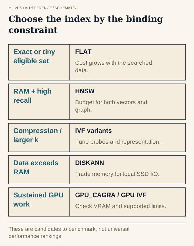 Choose the index by the binding constraint. These are candidates to benchmark, not universal performance rankings.
Step 1: Describe the workload before you look at indexes
Index choice depends far more on the workload than on the vector count alone. Write these down first:
- Field type and metric. Dense float (also FP16, BF16, INT8), binary, or sparse vectors each have their own index families. The metric (COSINE, L2, IP for dense; HAMMING or JACCARD for binary; IP or BM25 for sparse) must match how the embedding was trained.
- Size and dimension, now and in a year. Raw memory is
N × d × bytes per value. One million 768-dimensional FP32 vectors is about 3 GB before any index overhead. - Memory, SSD, and GPU budget per query node.
- Recall target at your
k, measured against exact search. - Latency SLO and concurrency, e.g. p99 under 20 ms at 500 QPS.
- Top-k size. Ten results and ten thousand results favour different structures.
- Filter selectivity: what fraction of the collection a typical filter removes.
- Write pattern: append-only, constant upserts, or periodic bulk reloads.
Step 2: Know what each Milvus index actually does
This is the reference table for the whole family. Each index is a combination of a candidate-selection structure (scan, clusters, graph) and a vector representation (full precision or compressed).
| Index | Structure + representation | Key parameters | Memory (relative to raw vectors) | Best fit | Watch out for |
|---|---|---|---|---|---|
FLAT | Exhaustive scan, full precision | none | 1× | Small or heavily filtered sets; ground truth | Cost grows linearly with N × d |
IVF_FLAT | k-means clusters, full vectors | nlist (build), nprobe (search) | ≈1× + centroids | Balanced default when memory fits; large top-k | Recall depends on nprobe; clusters must be trained on representative data |
IVF_SQ8 | Clusters + 8-bit scalar codes | nlist, nprobe | ≈¼× | Memory-limited IVF with modest recall loss | Some precision loss |
IVF_PQ | Clusters + product-quantized codes | nlist, m, nbits, nprobe | Much smaller (e.g. 8× compression at m=64, nbits=8 for 128-d) | Very large collections on a tight memory budget | Lower recall unless refined; m must divide dim |
IVF_RABITQ | Clusters + ~1-bit RaBitQ codes, optional refine | nlist, refine, refine_type, nprobe, rbq_query_bits, refine_k | ≈1/32 of FP32 for codes, plus refine data | Maximum compression on modern CPUs | Benefits from AVX-512 VPOPCNTDQ; needs refine for high recall |
SCANN | Clusters + anisotropic quantization + reorder | nlist, with_raw_data, nprobe, reorder_k | Smaller codes; raw data kept by default | IVF-style search with stronger quantized scoring | reorder_k should be at least limit |
HNSW | Multi-layer proximity graph, full vectors | M, efConstruction (build), ef (search) | 1× + graph links | Low latency, high recall, data fits in RAM | Graph memory and build time; very selective filters |
HNSW_SQ / HNSW_PQ / HNSW_PRQ | HNSW graph + SQ / PQ / residual PQ codes | HNSW params + sq_type or PQ params, refine, refine_type, refine_k | Graph + compressed codes | HNSW latency with less memory | Approximate distances; tune refine |
DISKANN | Vamana graph and full vectors on SSD, PQ codes in RAM | MaxDegree, SearchListSize, PQCodeBudgetGBRatio; search_list, BeamWidthRatio | Small RAM fraction; most data on NVMe | Datasets far larger than RAM | Needs fast NVMe and queryNode.enableDisk; latency depends on I/O |
AISAQ | DiskANN-style graph with PQ data also on SSD | max_degree, search_list_size, inline_pq; search_list, beamwidth | Near-zero DRAM | Billion-scale on standard servers, relaxed latency | More disk reads per query |
GPU_CAGRA | GPU-optimized graph | intermediate_graph_degree, graph_degree, build_algo; itopk_size, search_width | ≈1.8× raw (GPU memory) | High-throughput or batched search on GPU | Top-k ≤ 1024; GPU build of Milvus required |
GPU_IVF_FLAT / GPU_IVF_PQ | IVF on GPU, full or PQ codes | nlist, nprobe (+ PQ params) | 1× / compressed | Batched IVF workloads on GPU | Top-k ≤ 256 (IVF_FLAT) or ≤ 1024 (IVF_PQ) |
GPU_BRUTE_FORCE | Exhaustive scan on GPU | none | 1× | Exact results at GPU speed | Linear cost; GPU memory |
BIN_FLAT / BIN_IVF_FLAT | Exact scan / IVF for binary vectors | nlist, nprobe for IVF | 1/32 of FP32 per dimension | Binary hashes and fingerprints | HAMMING or JACCARD |
MINHASH_LSH | LSH over binary MinHash signatures | mh_lsh_band, mh_element_bit_width, with_raw_data | Signatures + hash tables | Near-duplicate text detection | Metric must be MHJACCARD; not a dense-vector index |
SPARSE_INVERTED_INDEX | Inverted lists over non-zero dimensions | inverted_index_algo; for BM25 also bm25_k1, bm25_b | Proportional to non-zeros | Learned sparse embeddings and BM25 full-text search | Metric is IP, or BM25 for full-text fields |
For concrete numbers, the Milvus docs estimate that one million 128-dimensional vectors take about 515 MB with IVF_FLAT, 131 MB with IVF_SQ8, and about 11 MB with IVF_PQ (62 MB if 10% refinement data is kept); the same data in HNSW needs roughly 640 MB (graph plus vectors), while HNSW_PQ drops to about 136 MB. Graph links are the cost HNSW pays for its speed.
Step 3: Apply the decision rules
Work through these in order; the first rule that matches usually determines the family.
- Is it a sparse or binary field? Sparse →
SPARSE_INVERTED_INDEX(with metricBM25for full-text search). Binary →BIN_FLATfor exact,BIN_IVF_FLATfor speed,MINHASH_LSHfor MinHash near-duplicate detection. The remaining rules are for dense vectors. - Does the data fit in memory? If everything fits, use an in-memory index. If only about a quarter of the raw data fits in memory, Milvus suggests considering
DISKANN. In between, compressed indexes (HNSW_SQ,HNSW_PQ,IVF_PQ,IVF_RABITQ) or mmap can stretch capacity; Milvus recommends HNSW over IVF when mmap is enabled. - How selective are filters? Per the Milvus index guide, when filters remove less than about 85% of the data, graph indexes tend to win; between roughly 85% and 95%, IVF variants do better; and above about 98% filtered, the remaining set is small enough that
FLATgives exact results cheaply. - How large is top-k? Graph indexes are preferred for small top-k (up to around 2,000). When top-k approaches 1% of the dataset, or combines medium top-k with heavy filtering, IVF is usually more efficient.
- Is there a GPU, and enough traffic to keep it busy? Try
GPU_CAGRAfor graph search orGPU_IVF_FLAT/GPU_IVF_PQfor IVF, respecting their top-k limits. On low, bursty traffic a GPU often gives little advantage over a well-tuned CPU index. See GPU_CAGRA. - Otherwise, in memory with small top-k and a high recall target, start with
HNSW; with large result sets or a need for cheap compression, start withIVF_FLATand move toIVF_SQ8,IVF_PQ, orIVF_RABITQas memory requires.
Worked example
Suppose you have 50 million 768-dimensional FP32 embeddings for a RAG service: about 154 GB of raw vectors, top-10 queries, a 95% recall target, light tenant filters, and query nodes with 64 GB of RAM each.
- Plain
HNSWwould need the full 154 GB plus graph links in memory, i.e. several nodes just to hold one replica. HNSW_SQwithsq_typeSQ8 cuts vector memory roughly 4×, to under 40 GB plus graph, which fits on a node or two. Turn onrefineif recall falls short.DISKANNkeeps only PQ codes in RAM (by defaultPQCodeBudgetGBRatiois 0.125 of the raw size, about 19 GB) and the rest on NVMe, trading a few milliseconds of SSD latency for a much smaller memory bill.
The shortlist is therefore HNSW_SQ versus DISKANN, benchmarked at the same 95% recall. If the filters were instead a strict per-user scope that leaves only a few thousand vectors per query, FLAT on a partition-key-scoped search could beat both.
Step 4: Compare candidates at equal recall under real load
An index decision is only as good as the benchmark behind it:
- Compute exact neighbors with
FLATon the same data, metric, filters, andk, and report Recall@k against that (why use a FLAT baseline). Track application relevance separately. - For each index, fix build parameters and sweep the search parameter (
ef,nprobe,search_list), then compare latency at the same recall, not each index at its best-case setting. - Record p50/p95/p99 latency at realistic concurrency, QPS, build and load time, resident memory, disk I/O or GPU use, and behaviour during writes and compaction.
- Repeat when the embedding model, data distribution, filters, hardware, or Milvus version change. Supported index types and parameters vary by release, so check the versioned docs for your deployment.
Compression is a second decision layered on the first: choose how candidates are found, then how vectors are stored. A refine step can reorder retrieved candidates with higher precision, but it cannot recover a neighbor the search never reached. The quantization guide and HNSW_SQ, HNSW_PQ, and HNSW_PRQ trade-offs cover that layer in detail.
Next steps in Milvus
Create a collection with AUTOINDEX in the Milvus Quickstart, then rebuild with an explicit index type once you have a benchmark. If you would rather not size nodes and indexes yourself, Zilliz Cloud runs managed Milvus with automatic index selection.
Related reading
- What is approximate nearest-neighbor search?
- What is HNSW, and how should you tune it?
- How do IVF indexes use centroids to search vectors?
- When should you use DISKANN in Milvus?
- How do you estimate memory for vector search?
- What is FAISS, and how does it relate to vector indexes?
Sources
- Milvus index explained: types, memory estimates, selection advice
- Milvus index selection guide
- HNSW, HNSW_SQ, IVF_FLAT, IVF_PQ, IVF_RABITQ, SCANN
- DISKANN and AISAQ
- GPU indexes and GPU_CAGRA
- BIN_FLAT, sparse vectors, full-text search
- Memory mapping (mmap)
- Aumüller et al., ANN-Benchmarks (arXiv:1807.05614)


