Beyond the TurboQuant-RaBitQ Debate: Why Vector Quantization Matters for AI Infrastructure Costs

Google’s TurboQuant paper (ICLR 2026) reported 6x KV cache compression with near-zero accuracy loss — results striking enough to wipe $90 billion off memory chip stocks in a single day. SK Hynix dropped 12%. Samsung dropped 7%.

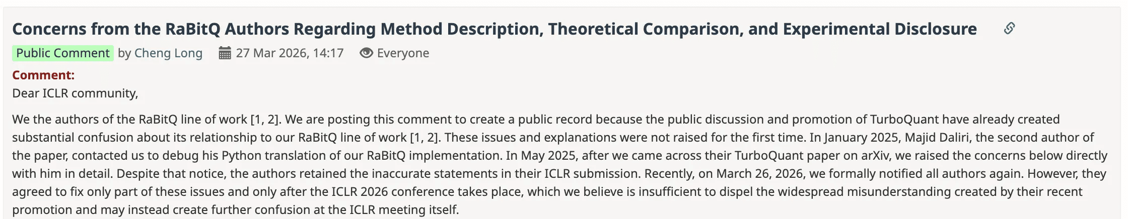
The paper quickly drew scrutiny. Jianyang Gao, first author of RaBitQ (SIGMOD 2024), raised questions about the relationship between TurboQuant’s methodology and his prior work on vector quantization. (We’ll be publishing a conversation with Dr. Gao soon — follow us if you’re interested.)

This article isn’t about taking sides in that discussion. What struck us is something bigger: the fact that a single vector quantization paper could move $90 billion in market value tells you how critical this technology has become for AI infrastructure. Whether it’s compressing KV cache in inference engines or compressing indexes in vector databases, the ability to shrink high-dimensional data while preserving quality has enormous cost implications — and it’s a problem we’ve been working on, integrating RaBitQ into Milvus vector database and turning it into production infrastructure.

Here’s what we’ll cover: why vector quantization matters so much right now, how TurboQuant and RaBitQ compare, what RaBitQ is and how it works, the engineering work behind shipping it inside Milvus, and what the broader memory optimization landscape looks like for AI infrastructure.

Why Does Vector Quantization Matter for Infrastructure Costs?

Vector quantization is not new. What’s new is how urgently the industry needs it. Over the past two years, LLM parameters have ballooned, context windows have stretched from 4K to 128K+ tokens, and unstructured data — text, images, audio, video — has become a first-class input to AI systems. Every one of these trends creates more high-dimensional vectors that need to be stored, indexed, and searched. More vectors, more memory, more cost.

If you’re running vector search at scale — RAG pipelines, recommendation engines, multimodal retrieval — memory cost is likely one of your biggest infrastructure headache.

During model deployment, every major LLM inference stack relies on KV cache — storing previously computed key-value pairs so the attention mechanism doesn’t recompute them for every new token. It’s what makes O(n) inference possible instead of O(n²). Every framework from vLLM to TensorRT-LLM depends on it. But KV cache can consume more GPU memory than the model weights themselves. Longer contexts, more concurrent users, and it spirals fast.

The same pressure hits vector databases — billions of high-dimensional vectors sitting in memory, each one a 32-bit float per dimension. Vector quantization compresses these vectors from 32-bit floats down to 4-bit, 2-bit, or even 1-bit representations — shrinking memory by 90% or more. Whether it’s KV cache in your inference engine or indexes in your vector database, the underlying math is the same, and the cost savings are real. That’s why a single paper reporting a breakthrough in this space moved $90 billion in stock market value.

TurboQuant vs RaBitQ: What’s the Difference?

Both TurboQuant and RaBitQ build on the same foundational technique: applying a random rotation (Johnson-Lindenstrauss transform) to input vectors before quantization. This rotation transforms irregularly distributed data into a predictable uniform distribution, making it easier to quantize with low error.

Beyond that shared foundation, the two target different problems and take different approaches:

	TurboQuant	RaBitQ
Target	KV cache in LLM inference (ephemeral, per-request data)	Persistent vector indexes in databases (stored data)
Approach	Two-stage: PolarQuant (Lloyd-Max scalar quantizer per coordinate) + QJL (1-bit residual correction)	Single-stage: hypercube projection + unbiased distance estimator
Bit width	3-bit keys, 2-bit values (mixed precision)	1-bit per dimension (with multi-bit variants available)
Theoretical claim	Near-optimal MSE distortion rate	Asymptotically optimal inner-product estimation error (matching Alon-Klartag lower bounds)
Production status	Community implementations; no official release from Google	Shipped in Milvus 2.6, adopted by Faiss, VSAG, Elasticsearch

The key difference for practitioners: TurboQuant optimizes the transient KV cache inside an inference engine, while RaBitQ targets the persistent indexes that a vector database builds, shards, and queries across billions of vectors. For the rest of this article, we’ll focus on RaBitQ — the algorithm we’ve integrated and ship in production inside Milvus.

What Is RaBitQ and What Does It Deliver?

Here’s the bottom line first: on a 10-million vector dataset at 768 dimensions, RaBitQ compresses each vector to 1/32 of its original size while keeping recall above 94%. In Milvus, that translates to 3.6x higher query throughput than a full-precision index. This isn’t a theoretical projection — it’s a benchmark result from Milvus 2.6.

Now, how it gets there.

Traditional binary quantization compresses FP32 vectors to 1 bit per dimension — 32x compression. The tradeoff: recall collapses because you’ve thrown away too much information. RaBitQ (Gao & Long, SIGMOD 2024) keeps the same 32x compression but preserves the information that actually matters for search. An extended version (Gao & Long, SIGMOD 2025) proves this is asymptotically optimal, matching the theoretical lower bounds established by Alon & Klartag (FOCS 2017).

Why Do Angles Matter More Than Coordinates in High Dimensions?

The key insight: in high dimensions, angles between vectors are more stable and informative than individual coordinate values. This is a consequence of measure concentration — the same phenomenon that makes Johnson-Lindenstrauss random projections work.

What this means in practice: you can discard the exact coordinate values of a high-dimensional vector and keep only its direction relative to the dataset. The angular relationships — which is what nearest-neighbor search actually depends on — survive the compression.

How Does RaBitQ Work?

RaBitQ turns this geometric insight into three steps:

Step 1: Normalize. Center each vector relative to the dataset centroid and scale to unit length. This converts the problem to inner-product estimation between unit vectors — easier to analyze and bound.

Step 2: Random rotation + hypercube projection. Apply a random orthogonal matrix (a Johnson-Lindenstrauss-type rotation) to remove bias toward any axis. Project each rotated vector onto the nearest vertex of a {±1/√D}^D hypercube. Each dimension collapses to a single bit. The result: a D-bit binary code per vector.

Step 3: Unbiased distance estimation. Construct an estimator for the inner product between a query and the original (unquantized) vector. The estimator is provably unbiased with error bounded by O(1/√D). For 768-dimensional vectors, this keeps recall above 94%.

Distance computation between binary vectors reduces to bitwise AND + popcount — operations modern CPUs execute in a single cycle. This is what makes RaBitQ fast, not just small.

Why Is RaBitQ Practical, Not Just Theoretical?

• No training required. Apply the rotation, check signs. No iterative optimization, no codebook learning. Indexing time is comparable to product quantization.
• Hardware-friendly. Distance computation is bitwise AND + popcount. Modern CPUs (Intel IceLake+, AMD Zen 4+) have dedicated AVX512VPOPCNTDQ instructions. Single-vector estimation runs 3x faster than PQ lookup tables.
• Multi-bit flexibility. The RaBitQ Library supports variants beyond 1-bit: 4-bit achieves ~90% recall, 5-bit ~95%, 7-bit ~99% — all without reranking.
• Composable. Plugs into existing index structures like IVF indexes and HNSW graphs, and works with FastScan for batch distance computation.

From Paper to Production: What We Built to Ship RaBitQ in Milvus

The original RaBitQ code is a single-machine research prototype. Making it work across a distributed cluster with sharding, failover, and real-time ingestion required solving four engineering problems. At Zilliz, we went beyond simply implementing the algorithm — the work spanned engine integration, hardware acceleration, index optimization, and runtime tuning to turn RaBitQ into an industrial-grade capability inside Milvus. You can find more details in this blog as well: Bring Vector Compression to the Extreme: How Milvus Serves 3× More Queries with RaBitQ

Making RaBitQ Distributed-Ready

We integrated RaBitQ directly into Knowhere, Milvus’s core search engine — not as a plugin, but as a native index type with unified interfaces. It works with Milvus’s full distributed architecture: sharding, partitioning, dynamic scaling, and collection management.

The key challenge: making the quantization codebook (rotation matrix, centroid vectors, scaling parameters) segment-aware, so that each shard builds and stores its own quantization state. Index builds, compactions, and load-balancing all understand the new index type natively.

Squeezing Every Cycle Out of Popcount

RaBitQ’s speed comes from popcount — counting set bits in binary vectors. The algorithm is inherently fast, but how much throughput you get depends on how well you use the hardware. We built dedicated SIMD code paths for both dominant server architectures:

• x86 (Intel IceLake+ / AMD Zen 4+): AVX-512’s VPOPCNTDQ instruction computes popcount across multiple 512-bit registers in parallel. Knowhere’s inner loops are restructured to batch binary distance computations into SIMD-width chunks, maximizing throughput.
• ARM (Graviton, Ampere): SVE (Scalable Vector Extension) instructions for the same parallel popcount pattern — critical since ARM instances are increasingly common in cost-optimized cloud deployments.

Eliminating Runtime Overhead

RaBitQ needs auxiliary floating-point parameters at query time: the dataset centroid, per-vector norms, and the inner product between each quantized vector and its original (used by the distance estimator). Computing these per query adds latency. Storing the full original vectors defeats the purpose of compression.

Our solution: pre-compute and persist these parameters during index build, caching them alongside the binary codes. The memory overhead is small (a few floats per vector), but it eliminates per-query computation and keeps latency stable under high concurrency.

IVF_RABITQ: The Index You Actually Deploy

Starting with Milvus 2.6, we ship IVF_RABITQ — Inverted File Index + RaBitQ quantization. The search works in two stages:

1. Coarse search (IVF). K-means partitions the vector space into clusters. At query time, only the nprobe closest clusters are scanned.
2. Fine scoring (RaBitQ). Within each cluster, distances are estimated using 1-bit codes and the unbiased estimator. Popcount does the heavy lifting.

The results on a 768-dimensional, 10-million vector dataset:

Metric	IVF_FLAT (baseline)	IVF_RABITQ	IVF_RABITQ + SQ8 refine
Recall	95.2%	94.7%	~95%
QPS	236	864	—
Memory footprint	32 bits/dim	1 bit/dim (~3% of original)	~25% of original

For workloads that can’t tolerate even a 0.5% recall gap, the refine_type parameter adds a second scoring pass: SQ6, SQ8, FP16, BF16, or FP32. SQ8 is the common choice — it restores recall to IVF_FLAT levels at roughly 1/4 the original memory. You can also apply scalar quantization to the query side (SQ1–SQ8) independently, giving you two knobs to tune the latency-recall-cost tradeoff per workload.

How Milvus Optimizes Memory Beyond Quantization

RaBitQ is the most dramatic compression lever, but it’s one layer in a broader memory optimization stack:

Strategy	What it does	Impact
Full-stack quantization	SQ8, PQ, RaBitQ at different precision-cost tradeoffs	4x to 32x memory reduction
Index structure optimization	HNSW graph compaction, DiskANN SSD offloading, OOM-safe index builds	Less DRAM per index, larger datasets per node
Memory-mapped I/O (mmap)	Maps vector files to disk, loads pages on demand via OS page cache	TB-scale datasets without loading everything into RAM
Tiered storage	Hot/warm/cold data separation with automatic scheduling	Pay memory prices only for frequently accessed data
Cloud-native scaling (Zilliz Cloud, managed Milvus)	Elastic memory allocation, auto-release of idle resources	Pay only for what you use

Full-Stack Quantization

RaBitQ’s 1-bit extreme compression isn’t the right fit for every workload. Milvus offers a complete quantization matrix: SQ8 and product quantization (PQ) for workloads that need a balanced precision-cost tradeoff, RaBitQ for maximum compression on ultra-large datasets, and hybrid configurations that combine multiple methods for fine-grained control.

Index Structure Optimization

Beyond quantization, Milvus continuously optimizes memory overhead in its core index structures. For HNSW, we reduced adjacency list redundancy to lower per-graph memory usage. DiskANN pushes both vector data and index structures to SSD, dramatically reducing DRAM dependency for large datasets. We also optimized intermediate memory allocation during index building to prevent OOM failures when building indexes over datasets that approach node memory limits.

Smart Memory Loading

Milvus’s mmap (memory-mapped I/O) support maps vector data to disk files, relying on the OS page cache for on-demand loading — no need to load all data into memory at startup. Combined with lazy loading and segmented loading strategies that prevent sudden memory spikes, this enables smooth operation with TB-scale vector datasets at a fraction of the memory cost.

Tiered Storage

Milvus’s three-tier storage architecture spans memory, SSD, and object storage: hot data stays in memory for low latency, warm data is cached on SSD for a balance of performance and cost, and cold data sinks to object storage to minimize overhead. The system handles data scheduling automatically — no application-layer changes required.

Cloud-Native Scaling

Under Milvus’s distributed architecture, data sharding and load balancing prevent single-node memory overload. Memory pooling reduces fragmentation and improves utilization. Zilliz Cloud (fully managed Milvus) takes this further with elastic scheduling for on-demand memory scaling — in Serverless mode, idle resources are automatically released, further reducing total cost of ownership.

How These Layers Compound

These optimizations aren’t alternatives — they stack. RaBitQ shrinks the vectors. DiskANN keeps the index on SSD. Mmap avoids loading cold data into memory. Tiered storage pushes archival data to object storage. The result: a deployment serving billions of vectors doesn’t need billions-of-vectors worth of RAM.

Get Started

As AI data volumes continue to grow, vector database efficiency and cost will directly determine how far AI applications can scale. We’ll continue investing in high-performance, low-cost vector infrastructure — so that more AI applications can move from prototype to production.

Milvus is open source. To try IVF_RABITQ:

• Check the IVF_RABITQ documentation for configuration and tuning guidance.
• Read the full RaBitQ integration blog post for deeper benchmarks and implementation details.
• Join the Milvus Slack community to ask questions and learn from other developers.
• Book a free Milvus Office Hours session to walk through your use case.

If you’d rather skip infrastructure setup, Zilliz Cloud (fully managed Milvus) offers a free tier with IVF_RABITQ support.

We’re running an upcoming interview with Professor Cheng Long (NTU, VectorDB@NTU) and Dr. Jianyang Gao (ETH Zurich), the first author of RaBitQ, where we’ll go deeper into vector quantization theory and what’s next. Drop your questions in the comments.

Frequently Asked Questions

What are TurboQuant and RaBitQ?

TurboQuant (Google, ICLR 2026) and RaBitQ (Gao & Long, SIGMOD 2024) are both vector quantization methods that use random rotation to compress high-dimensional vectors. TurboQuant targets KV cache compression in LLM inference, while RaBitQ targets persistent vector indexes in databases. Both have contributed to the current wave of interest in vector quantization, though they solve different problems for different systems.

How does RaBitQ achieve 1-bit quantization without destroying recall?

RaBitQ exploits measure concentration in high-dimensional spaces: the angles between vectors are more stable than individual coordinate values as dimensionality increases. It normalizes vectors relative to the dataset centroid, then projects each one onto the nearest vertex of a hypercube (reducing each dimension to a single bit). An unbiased distance estimator with a provable error bound keeps search accurate despite the compression.

What is IVF_RABITQ and when should I use it?

IVF_RABITQ is a vector index type in Milvus (available since version 2.6) that combines inverted file clustering with RaBitQ 1-bit quantization. It achieves 94.7% recall at 3.6x the throughput of IVF_FLAT, with memory usage at roughly 1/32 of the original vectors. Use it when you need to serve large-scale vector search (millions to billions of vectors) and memory cost is a primary concern — common in RAG, recommendation, and multimodal search workloads.

How does vector quantization relate to KV cache compression in LLMs?

Both problems involve compressing high-dimensional floating-point vectors. KV cache stores key-value pairs from the Transformer attention mechanism; at long context lengths, it can exceed the model weights in memory usage. Vector quantization techniques like RaBitQ reduce these vectors to lower-bit representations. The same mathematical principles — measure concentration, random rotation, unbiased distance estimation — apply whether you’re compressing vectors in a database index or in an inference engine’s KV cache.