SVS in Milvus: Reshaping the Recall–Memory–Speed Trade-off

Every production vector index forces the same trade-off at search time: high recall, a small memory footprint, and fast queries — you rarely get all three at once. Push recall up, and you usually pay for it, in memory (you drop the compression) or in latency (you widen the search window until throughput collapses). And that’s just at search time — building the index is a cost of its own, especially for graph indexes. Milvus’s cost-optimization guide lays the trade-off out plainly: for cost-sensitive workloads it recommends IVF_SQ8 for its ~4× memory savings, and flags HNSW as the memory-hungry choice you reach for “only when latency matters more than cost.”

But plenty of production workloads do need HNSW-class speed and recall — RAG pipelines, agentic retrieval, and recommendation systems are all sensitive to what’s missing from the top-k, and increasingly want to push recall past the ~95% that quantized HNSW comfortably delivers. The usual way to take the edge off HNSW’s memory cost is scalar quantization: HNSW_SQ (backed by Faiss) with SQ8 quantizes each dimension to 8 bits, which gets you fast, ~95% recall search at a fraction of full-precision memory. That’s the pragmatic high-performance baseline most teams settle on — and it’s the one that starts to crack the moment you need more than 95% recall.

SVS Vamana, a new index in Milvus built on Intel’s Scalable Vector Search (SVS) library, changes the calculus. With LeanVec compression enabled — we’ll call this SVS LeanVec — its recall-vs-QPS curve sits above both HNSW SQ8 and HNSW FP16 across the whole operating range — more throughput and lower latency at any given recall, with the lead widening as you push recall higher, all while staying well clear of FP16’s memory cost. It significantly shifts the recall / memory / performance trade-off most teams treat as fixed.

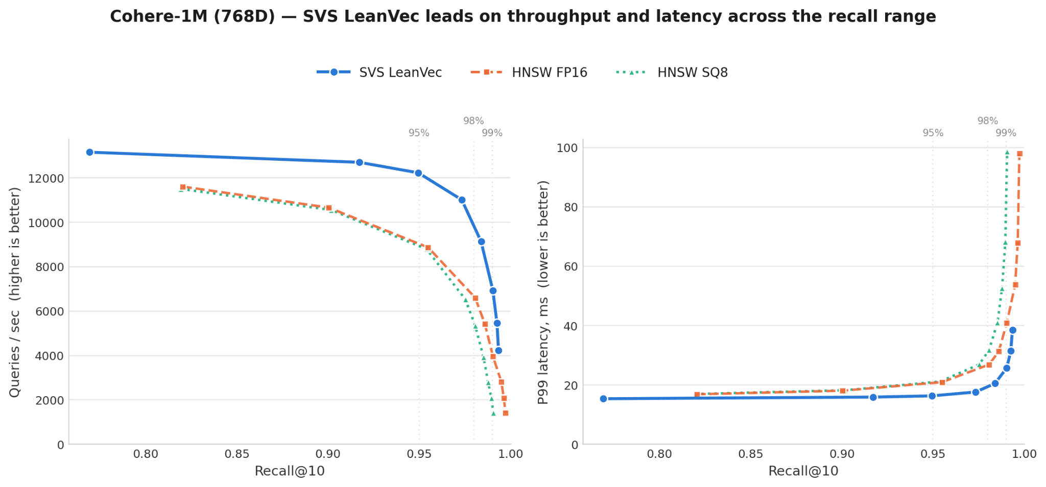
Cohere-1M, k=10: SVS LeanVec leads on throughput (left, higher is better) and latency (right, lower is better) across the entire recall range.

This post walks through what SVS Vamana and LeanVec actually do, why memory is the axis that decides your bill, and then shows the numbers across four datasets on the metrics that matter in production: queries per second, P99 latency, load time, memory footprint, and the one that ties them together, throughput per gigabyte.

Why This Trade-off Is Really a Cost Problem

Recall, memory, and speed are entangled because it comes down to cost. For an in-memory vector index, memory is where the bill goes — that same cost-optimization guide puts 85–90% of your spend there, since keeping vectors and their graph resident in RAM is what makes search fast. So the levers are simple:

• Compress harder → cheaper, but recall drops unless you widen the search.
• Widen the search → recall recovers, but latency and cost-per-query climb.
• Store in full precision → recall is easy, but memory — and the bill — balloons.

At 95% recall, you can escape that trap with HNSW SQ8. Above 95%, quantized HNSW forces you back toward full-precision storage or impractically wide searches. SVS LeanVec compresses the thing you traverse very aggressively while keeping the thing you re-rank with faithful enough to recover accuracy — and it does that with quantized vectors throughout, never a full-precision copy. Here’s how.

What Is SVS Vamana?

SVS Vamana builds on a Vamana graph — the same in-memory proximity graph behind DiskANN, pruned so that search “jumps” toward the query in a few long-range hops instead of crawling neighbor-to-neighbor. That alone makes it a solid graph index. What makes it compelling for memory-constrained production is the compression layered on top: LeanVec.

LeanVec: dimensionality reduction and quantization, together

LeanVec compresses vectors two ways at once:

• Dimensionality reduction. Each vector gets a linear projection down to a fraction of its original dimensionality — a half, a quarter, a sixth, whatever you configure. The Vamana graph is built and searched over this reduced primary representation, so most distance computations during traversal happen in a much smaller space.
• Quantization. Both the reduced primary vectors and a full-dimensional secondary copy are compressed with LVQ (Locally-adaptive Vector Quantization) — typically 4 bits per dimension for the primary structure that does the heavy lifting during traversal, and 8 bits per dimension for the secondary structure used to re-rank the final candidates and recover the accuracy lost to dimensionality reduction. Note that the secondary copy is full-dimensional but still quantized — LeanVec never keeps a float32 full-precision copy. That 8-bit-per-dimension secondary is already ~4× smaller than the original float32 embedding; it’s “high fidelity” only relative to the aggressively compressed primary, not full precision.

Here’s the key intuition, and the mechanism behind every number below. SQ8 shrinks every dimension to 8 bits but still searches the full-dimensional vector on every hop. LeanVec searches a much smaller, lower-dimensional vector on every hop, and re-ranks the small surviving candidate set against the full-dimensional (but still 8-bit) secondary copy. Less data through memory on the hot path, and even the re-ranking pass never touches a full-precision vector — that’s how it’s simultaneously faster, smaller, and high on the recall curve.

By default, LeanVec uses an out-of-distribution (OOD) mode that learns two projections — one for the base vectors, one for the queries — rather than the single shared projection of the simpler in-distribution (ID) build. That extra flexibility shines when queries and indexed vectors follow different distributions (cross-modal text-to-image being the canonical case), and it helps in-distribution too. OOD costs some extra build time, so you can switch to the ID build when build speed matters more; we benchmark both.

Hardware note: LVQ and LeanVec compression run on any Intel CPU, and are much faster with AVX-512 — recommended for best performance, which currently requires a 2nd-gen Xeon or newer (we used Xeon 6). SVS Vamana itself isn't Intel-only: its FP32, FP16, and SQ8 storage kinds run anywhere (SQ8 here is plain 8-bit scalar quantization), so you can build the Vamana graph on any platform and add LVQ/LeanVec on Intel. All results here use SVS LeanVec.

Trying It in Milvus

That’s the mechanism — here’s how to put it to work. Creating the index looks like any other Milvus index:

from pymilvus import MilvusClient

index_params = MilvusClient.prepare_index_params()

index_params.add_index(
    field_name="your_vector_field_name",
    index_type="FAISS",
    index_name="vector_index",
    metric_type="L2",
    params={
        # SVSVamana64 -> Vamana graph degree 64
        # LeanVec4x8  -> 4-bit primary, 8-bit secondary
        # _128        -> LeanVec dim 128 (omit the suffix for dim / 2)
        "faiss_index_name": "SVSVamana64,LeanVec4x8_128",
        "construction_window_size": 200,  # build-time search width
        "ood_training": True,             # OOD on (default); set False for faster builds
    }
)

At search time, search_window_size controls the recall/latency trade-off, exactly the way ef does for HNSW. Additionally, search_buffer_capacity must be at least search_window_size.

search_params = {
    "params": {
        "search_window_size": 100,      # wider = higher recall, lower QPS
        "search_buffer_capacity": 100,  # must be at least search_window_size
    }
}

res = MilvusClient.search(
    collection_name="your_collection_name",
    anns_field="vector_field",
    data=[[0.1, 0.2, 0.3, 0.4, 0.5]],
    limit=10,
    search_params=search_params,
)

See the SVS Vamana index docs for the full parameter reference — graph construction tuning, OOD, and the other storage kinds (FP32, FP16, SQ8 for uncompressed SVS Vamana; LVQ4x0/LVQ4x4/LVQ4x8 for LVQ quantization without dimensionality reduction).

Enabling SVS. SVS support is not enabled in the default Milvus images, so build Milvus from source with make milvus USE_SVS=ON to try it.

Picking a storage kind. LeanVec4x8 is a good default — dimensionality reduction plus 4-bit/8-bit LVQ — and it’s what we benchmark here. From there:

• Want more recall / higher fidelity (at some memory cost)? Use LVQ without dimensionality reduction (LVQ4x8), or raise the LeanVec dim (the _N suffix in the factory string).
• Want a smaller footprint (at some recall cost)? Go more aggressive — a lower LeanVec dim, a 4-bit secondary (LeanVec4x4), or a 4-bit LVQ with no secondary (LVQ4x0).
• Not on Intel? Use FP16 or SQ8.

The Setup

We benchmarked SVS LeanVec (LeanVec4x8 storage — 4-bit primary, 8-bit secondary — both with and without OOD, at several search-window sizes) against Milvus’s Faiss-backed HNSW_SQ index in both its FP16 and SQ8 scalar-quantization storage modes, across four dataset/scale combinations:

Dataset	Dimensions	Vectors
Cohere	768	1M
Bioasq	1024	1M
OpenAI	1536	500K
OpenAI	1536	5M

For each dataset, we swept every index’s search parameters across a range of recall values — tracing the full recall-vs-QPS curves — at both k=10 and k=100. We measured index load time, queries per second (QPS), and P99 latency, at a fixed concurrency of 100 client threads.

We use HNSW’s 16-bit FP16 mode as the heavyweight baseline rather than uncompressed 32-bit FP32. FP32 stores twice the bytes per vector (≈2× FP16’s memory) with no search-throughput benefit and essentially identical recall, so FP16 is the stronger, more cost-competitive HNSW to compare against — SVS’s memory lead over plain FP32 HNSW would only be wider.

Setup details. SVS builds used a Vamana graph max degree of 64 (construction window 200) and a LeanVec dim of 256 (Cohere, OpenAI) / 512 (Bioasq); HNSW used M=32 (up to 2M = 64 neighbors per node in its base layer) and efConstruction=200 — so SVS’s single-layer Vamana graph at max degree 64 matches HNSW’s base-layer connectivity. All indexes used the COSINE metric. We ran everything with VectorDBBench: Milvus on an AWS r8id.4xlarge server (16 vCPUs, Intel Xeon 6, 128 GiB RAM, 950 GB NVMe SSD), driven by a c8i.4xlarge client (16 vCPUs, Intel Xeon 6). Milvus 3.0 (pre-release, commit 67c0a23f5a).

The Full Recall–QPS Picture

The figure in the intro is Cohere; the same pattern holds across all four datasets and the whole recall range. The tables and figures that follow are at k=10; we also evaluated k=100, which tells the same story — SVS LeanVec on top across the recall range. The SVS numbers use LeanVec with OOD on. OOD improves query throughput over the faster-to-build in-distribution (ID) variant — a small edge at ~95% recall that widens at higher targets (and larger still on cross-modal data) — in exchange for extra build time (see Load Time). The overall comparison holds either way; the margins here are with OOD on. Start at a mainstream operating point — around 95% recall — where SVS LeanVec already beats HNSW SQ8, the cheapest HNSW configuration, on every dataset, on both QPS and P99 latency:

Dataset	HNSW SQ8 QPS	HNSW SQ8 P99	SVS LeanVec QPS	SVS LeanVec P99	QPS gain	Latency cut
Cohere 1M (768D)	8,723	21.15 ms	12,233	16.08 ms	×1.40	−24%
Bioasq 1M (1024D)	3,637	42.93 ms	6,691	26.54 ms	×1.84	−38%
OpenAI 500K (1536D)	7,367	23.95 ms	10,828	17.83 ms	×1.47	−26%
OpenAI 5M (1536D)	3,610	42.50 ms	6,595	26.65 ms	×1.83	−37%

All recall values calibrated to 95% at k=10; concurrency = 100.

Key findings:

• Up to ×1.84 more QPS and up to −38% P99 latency vs. HNSW SQ8, at the same 95% recall.
• The gains are largest on the higher-dimensional and larger-scale datasets (Bioasq 1024D, OpenAI 5M) — exactly where the cost of moving full-dimensionality vectors through memory bites hardest, and exactly where LeanVec’s dimensionality reduction pays off most.
• SVS LeanVec also outran HNSW FP16 on every dataset here — despite FP16 storing every dimension at 16 bits with no dimensionality reduction at all.

But 95% is just one point on the curve — and the SVS advantage grows as you demand higher recall. As the intro figure shows, SVS LeanVec’s throughput declines gently as recall rises while quantized HNSW SQ8’s falls off a cliff. The Cohere-1M numbers make the divergence concrete:

Recall target	HNSW SQ8 QPS	HNSW SQ8 P99	SVS LeanVec QPS	SVS LeanVec P99
95%	8,723	21.15 ms	12,233	16.08 ms
98%	5,266	32.44 ms	10,167	18.45 ms
99%	1,590	86.23 ms	7,252	24.59 ms

The SVS advantage grows from ×1.4 at 95% recall to ×1.9 at 98% and ×4.6 at 99%. By 99%, HNSW SQ8’s throughput has collapsed to roughly a fifth of its 95% number and its P99 latency has more than quadrupled — the search window it needs on quantized vectors is that wide — while SVS LeanVec has given up far less.

The same pattern holds across datasets, and on the larger, higher-dimensional ones it’s starker still: at the search settings used here, HNSW SQ8’s throughput collapses as it approaches the top of the recall range, stalling below the highest targets on OpenAI-500K, OpenAI-5M, and Bioasq. OpenAI-5M shows it clearly:

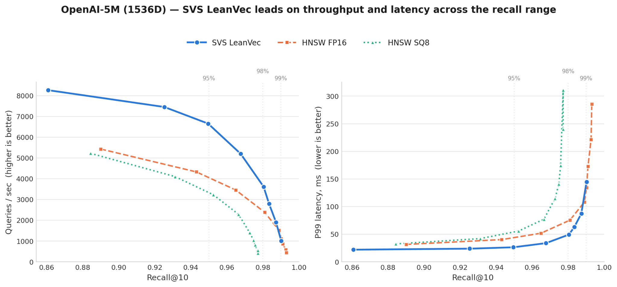
OpenAI-5M (1536D, 5M), k=10: SVS LeanVec leads on throughput (left) and latency (right) across the recall range; HNSW SQ8 trails throughout, and HNSW FP16 closes the gap only at the very highest recall (more on that below).

That leaves HNSW FP16 as the higher-fidelity alternative — but it carries HNSW’s full 16-bit-per-dimension memory cost, and SVS matches or beats it even there:

• Cohere 1M, 99%: SVS LeanVec holds 7,252 QPS vs. FP16’s 4,873 — a 49% QPS lead and 28% lower P99 latency.
• OpenAI 500K, 99%: SVS LeanVec 4,523 QPS / 35.95 ms P99 vs. FP16 3,868 QPS / 42.14 ms — ahead on both.
• OpenAI 5M, 99%: the one case where FP16 wins (1,186 QPS / 114.28 ms vs. 1,011 QPS / 131.44 ms). The aggressive 6× dimensionality reduction we used needs a wide search window at this scale. SVS LeanVec exposes the LeanVec dim for exactly this — a gentler reduction (÷3 or ÷4 instead of ÷6) trades some memory back for speed, and is the first knob we’d turn here.

We flag that one exception deliberately: on OpenAI-5M at the very top of the range, FP16 edges ahead — a tunable LeanVec-dim knob, not a fundamental limit. Everywhere else, across the whole recall range, SVS LeanVec’s curve stays on top.

Bioasq is simply a hard dataset: at the graph max-degree used here, no index reaches 0.99 recall — not even HNSW FP16 — but across the range it does support, SVS LeanVec still leads on throughput and out-reaches HNSW SQ8.

These numbers are the end-to-end result of the full SVS LeanVec stack — the Vamana graph, LeanVec dimensionality reduction, and built-in refinement with LVQ quantization, in an x86-tuned implementation — not an attempt to isolate how much each piece contributes. What matters in practice is the combined effect, and these numbers reflect that.

The TCO Picture: Memory and Throughput per GiB

Speed is half the story; the other half is what it costs to keep that speed online — and as we noted up front, memory is where most of the bill goes. The rough per-vector footprint is easy to reason about (at dimensionality d): HNSW FP16 stores ~2·d bytes, HNSW SQ8 ~d, and LeanVec4x8 ~d/4 + d — so SVS should land well below FP16 and close to SQ8. On top of that, each graph index stores per-node neighbor lists (≈ out-degree × 4 bytes/node — the Vamana degree, or 2·M for HNSW): a dimension-independent cost that matters more at low d and fades at high dimensionality with modest M.

Here’s what we actually measured: the resident memory of the loaded index while serving queries — the number that sets your ongoing cost in Milvus, since it’s what each QueryNode holds in RAM, deciding how many vectors fit per node and multiplying with every replica you load.

Dataset	HNSW FP16	HNSW SQ8	SVS LeanVec (LeanVec4x8)	SVS vs. FP16
Cohere 1M (768D)	1.7 GiB	0.97 GiB	1.1 GiB	×0.65
Bioasq 1M (1024D)	2.2 GiB	1.2 GiB	1.5 GiB	×0.68
OpenAI 500K (1536D)	1.6 GiB	0.84 GiB	0.91 GiB	×0.57
OpenAI 5M (1536D)	15.6 GiB	8.4 GiB	9.0 GiB	×0.58

Resident memory of the vector index loaded and serving on the QueryNode (Milvus’s reported _vector_index_ metric), measured on the benchmark host. SVS config: _LeanVec4x8_, LeanVec dim = 256 (Cohere / OpenAI) and 512 (Bioasq).

One note on the transient: loading an index into a QueryNode briefly needs more than its resident footprint while the segment is brought into memory — but that overhead is proportionally similar across all three indexes, so the ranking is unchanged: SVS LeanVec’s peak while loading stays well below HNSW FP16’s, matching its steady-state footprint advantage.

Across every dataset, SVS LeanVec’s serving footprint is 57–68% of HNSW FP16’s — while matching or beating FP16 on throughput at every recall level — and sits in the same low-memory regime as HNSW SQ8 (within ~10–20% of it), the cheapest option. That’s the whole point: FP16-class-or-better speed at close-to-SQ8 memory.

Throughput per GiB: where speed and cost meet

What that footprint actually buys you is clearest when you divide throughput by it: queries per second per GiB of index — how much throughput each GiB of RAM buys you. Higher is cheaper. Here it is at 99% recall, where the memory and speed stories compound:

Dataset	HNSW FP16 (QPS/GiB)	HNSW SQ8 (QPS/GiB)	SVS LeanVec (QPS/GiB)	SVS vs. FP16
Cohere 1M (768D)	2,866	1,639	6,593	×2.3
OpenAI 500K (1536D)	2,418	stalls below 99%	4,970	×2.1
OpenAI 5M (1536D)	76	stalls below 99%	112	×1.5

QPS/GiB = (QPS at 99% recall, concurrency 100) ÷ (resident index memory in GiB). Bioasq is omitted here — no index reaches 99% recall on it (see the note above). SQ8 stalls below 99% on both OpenAI datasets.

SVS LeanVec delivers 1.5–2.3× more queries per second per GiB than HNSW FP16 at 99% recall. The metric flatters SVS not through arithmetic but because SVS is the only index here that’s simultaneously fast (numerator) and small (denominator) at high recall — FP16 is fast but memory-hungry; SQ8 is small but can’t reach 99% on most datasets. The clearest illustration is OpenAI-5M: even though FP16 posts slightly higher raw QPS there (1,186 vs 1,011), SVS still delivers ~1.5× more throughput per GiB, because it does it in 9.0 GiB instead of 15.6 GiB.

Load Time

One more practical dimension: build and load time. Because LeanVec builds a smaller, more compressed structure, SVS LeanVec also loads faster than HNSW — and its optional OOD mode lets you trade some of that build speed for better query performance, so we measured both settings. Check out the SVS Vamana documentation for details on disabling OOD mode to accelerate build performance when query throughput is less critical.

Dataset	HNSW FP16	HNSW SQ8	SVS LeanVec (no OOD)	SVS LeanVec OOD
Cohere 1M (768D)	740 s	740 s	521 s (×0.70)	716 s (×0.97)
Bioasq 1M (1024D)	791 s	831 s	620 s (×0.78)	1,532 s (×1.94)
OpenAI 500K (1536D)	621 s	621 s	390 s (×0.63)	658 s (×1.06)
OpenAI 5M (1536D)	6,270 s	7,650 s	3,811 s (×0.61)	6,326 s (×1.01)

Total build/load time; × values are relative to HNSW FP16. The query results elsewhere in this post use the OOD build.

Two clear patterns:

• With OOD off, SVS LeanVec loads 22–39% faster than HNSW on every dataset we tested — the direct benefit of building a smaller, lower-dimensional, more aggressively quantized structure.
• With OOD on, the picture is mixed — from about on par with HNSW (OpenAI-5M) to well above it on Bioasq (~1.9× HNSW FP16’s build time). OOD adds build-time work to improve the representation for faster queries — a real trade-off.

The upshot is a choice between the two LeanVec builds: LeanVec ID builds much faster than HNSW and delivers close to OOD’s query throughput at mainstream (~95%) recall, while OOD spends more build time to pull further ahead on queries — increasingly so at the highest recall targets. Reach for ID when build time matters or recall targets are moderate; reach for OOD when you want maximum query throughput at high recall.

Which Index Should You Actually Use?

Your situation	Use this	Why
~95% recall is enough, tightest memory budget	SVS LeanVec or HNSW SQ8	Both are cheap; SVS gives you more QPS and lower latency at the same recall and leaves you room to raise recall later without re-architecting.
You need 98–99% recall	SVS LeanVec	HNSW SQ8 either collapses in throughput or can’t calibrate to the target at all; SVS stays fast and gets there.
You’re on HNSW FP16 today for high recall	SVS LeanVec	Match or beat FP16 QPS/latency at a fraction of the memory — the clearest TCO win in our data.
Cross-modal / distribution-shifted queries	SVS LeanVec (OOD, the default)	OOD’s separate base/query projections help most when queries and indexed vectors follow different distributions.
Fastest builds, or recall around ~95%	SVS LeanVec with OOD off (ID)	Builds faster than the default, with near-OOD query performance at mainstream recall.
Very high recall at very large scale (multi-M, high-D)	SVS LeanVec, tune the LeanVec dim	A gentler dimensionality reduction trades a little memory back for throughput; the one place raw FP16 can still edge ahead.

Wrapping Up

The usual story with vector-index compression is “trade recall or latency for less memory — pick two.” SVS LeanVec significantly shifts that across most of the workloads we tested: it beats HNSW SQ8 at 95% recall and pulls further ahead as you push to higher recall, where quantized HNSW’s throughput falls off a cliff — and it stays faster than HNSW FP16, at a memory footprint near the cheap end of the scale, which is what governs how far and how affordably you can grow.

If you’re running HNSW today — quantized or not — and recall matters to you, SVS LeanVec is worth a side-by-side test on your own data. Grab the SVS Vamana docs to get started, and come tell us how it goes in the Milvus community — we read every benchmark you throw at us.

Acknowledgements

We would like to thank everyone at Intel and Zilliz who worked together to bring the Intel SVS library into Milvus. From Intel, this includes Andreas Huber, Dmitry Razdoburdin, Ethan Glaser, Igor Konopko, Rafik Saliev, and Yue Jiao; from Zilliz, Li Liu, Alexandr Guzhva, and the whole Knowhere and Milvus teams, who integrated and validated SVS in Knowhere and Milvus.