Hyperbolic Embeddings in Milvus

This is part 2 of a four-part series on hyperbolic embeddings in vector search: how to search them in Milvus and Zilliz Cloud with plain inner product, and when they’re worth using. This post runs it on Milvus and measures recall index by index. Part 1 explains why plain inner product works, part 3 runs it on Zilliz Cloud, and part 4 compares a hyperbolic model with CLIP.

Milvus has no hyperbolic distance metric, and it does not need one. As part 1 shows, two small changes are enough:

• At query time, flip the sign of the query vector’s first number. A plain inner-product search then returns exactly the hyperbolic ranking.
• At ingest, subtract the corpus average of that first number from every stored document (centering). The ranking doesn’t change, but the vectors index far better.

This post turns that into a Milvus deployment and measures it on the ImageNet dataset,^[1] about 1.28 million images, embedded with Hyper3-CLIP V1 (hyper3labs/hyper3-clip-v1). In short: with centering, a single inner-product search on HNSW matches the recall of a shortlist-and-rerank design, IVF indexes miss far fewer true neighbors, and the one index type to avoid is IVF_PQ.

A quick recap of the vectors. Each embedding is 513 numbers and sits on a bowl-shaped surface, the Lorentz hyperboloid. The first number is the point’s height up the bowl,^[2] which rises with its radius, the distance from the center. The other 512 say which direction the point lies in, and their overall size is the radius.

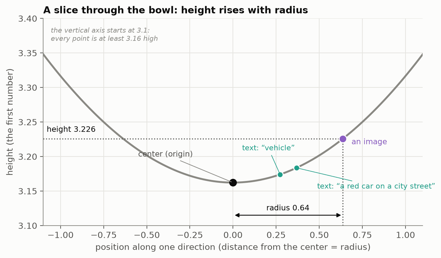The curve is the bowl seen side-on: move away from the center in any direction (horizontal axis) and the height, the first number, rises (vertical axis). The vertical axis starts at 3.1, which exaggerates the curve; every point is at least 3.16 high, which is why raw heights all sit around 3.2.

Two ways to deploy

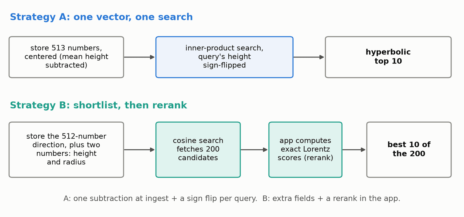The two deployments side by side. A is one vector and one search; B adds two scalar fields and a rerank over a 200-candidate shortlist.

Strategy A: one vector, one search. Store the 513-number vector, centered, and search with metric_type="IP" (inner product). One round trip (a single request to the database and back), no reranking, no extra fields.

m = float(corpus[:, 0].mean())         # once, at ingest
docs = corpus.copy(); docs[:, 0] -= m  # center documents only

q = np.array(emb, dtype=np.float32, copy=True)   # the query vector from the model
q[:, 0] *= -1.0                                  # flip the sign of the height
client.search(name, data=q.tolist(), anns_field="vec", limit=10,
              search_params={"metric_type": "IP"})

Never center the queries. Centering shifts every score for a given query by the same amount, so the top 10 is still exactly the hyperbolic top 10, but the scores Milvus returns are offset from the true Lorentz scores. If you need the true values, subtract $m$ multiplied by the query’s original height (before you flipped its sign). Keep $m$ with the collection, and center documents you add later with the same value.

Some implementations, such as HypRAG’s,^[3] flip the sign on the stored documents instead of the query. If you do that, center before flipping: store $-(y_0 - m)$.

The score Milvus returns, and how to convert it

With documents stored as $(y_0 - m, \bar{y})$ and the query sent as $(-x_0, \bar{x})$, Milvus returns

$$\text{score} = \langle x, y \rangle_L + x_0 m \qquad\Longrightarrow\qquad d(x, y) = \frac{\mathrm{arcosh}\left(-c\thinspace (\text{score} - x_0 m)\right)}{\sqrt{c}}$$

where $x_0$ is the query’s height before the sign flip and $c = 0.1$ for Hyper3-CLIP V1.

Strategy B: shortlist, then rerank. Store the 512-number direction, normalized to length 1, plus two scalar fields: h_time (the height) and h_radius (the radius). Run a cosine search to fetch a shortlist of candidates, then rerank them: compute each candidate’s exact Lorentz score in your application from the angle, the heights and the radii, and keep the best 10. hyper³labs’ own reference integration uses this shape.

The rerank formula

$$\langle x,y \rangle_L = -x_0 y_0 + \lVert \bar{x} \rVert \thinspace \lVert \bar{y} \rVert \cos\theta$$

where $x_0, y_0$ are the heights, $\lVert \bar{x} \rVert, \lVert \bar{y} \rVert$ the radii, and $\cos\theta$ the cosine similarity the search returns.

Or rerank inside Milvus. In Milvus 3.0.1 or later, a function chain can run that rerank in the database, so Strategy B also takes a single request, with no rerank code in your application. The chain multiplies each candidate’s stored radius by its cosine score, then adds the stored height, weighting the two by the query’s own radius and negated height:

from pymilvus.function_chain import FunctionChain, FunctionChainStage, col, fn

def lorentz_rerank(x0_q, r_q, k=10):
    return (FunctionChain(FunctionChainStage.L2_RERANK)
            .map("radius_cos", fn.num_combine(col("h_radius"), col("$score"), mode="multiply"))
            .map("$score", fn.num_combine(col("h_time"), col("radius_cos"), mode="weighted",
                                          weights=[-x0_q, r_q]))
            .sort("$score", desc=True)
            .limit(k))

client.search(name, data=[direction], anns_field="vec", limit=200,
              output_fields=["h_time", "h_radius"],
              search_params={"metric_type": "COSINE"},
              function_chains=lorentz_rerank(x0_q, r_q))

Here x0_q is the query’s height, r_q its radius and direction its other 512 numbers scaled to length 1. On 100 queries over 10,000 ImageNet images, the chain returned the same top 10 as the rerank in the application for every query, with scores within $5 \times 10^{-7}$. The weights belong to one query, so send one query per search request. Because the chain returns the same top 10, its recall is B’s; part 3 measures its latency on Zilliz Cloud.

On paper, A looks strictly better: it is simpler, and the database computes the exact hyperbolic score itself, with no rerank. The catch is that it only indexes well once the documents are centered (part 1 explains why centering is the fix, and why it keeps the ranking exact). So how well does it index?

Recall, index by index

We loaded the same 1.28 million vectors into Milvus v3.0.1 twice, once raw and once centered, then ran 1,000 text queries against each. For every query we computed the true top 10 by brute force, then measured recall@10: the share of those true top 10 that the index actually returned. We tested three index types:

• HNSW (Hierarchical Navigable Small World) builds a graph linking each vector to its near neighbors and searches by hopping through it. ef sets how many candidates it keeps in play while searching; higher is more accurate and slower.
• IVF_FLAT (inverted file) groups vectors into clusters and searches only the clusters nearest the query. nprobe sets how many clusters it searches.
• IVF_SQ8 is IVF with each number compressed to 8 bits (scalar quantization), cutting memory by about four times.

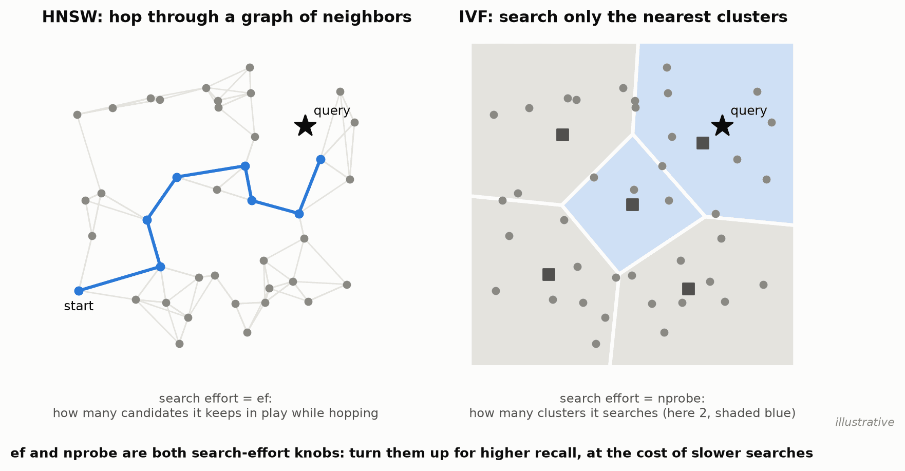How the two index families take shortcuts: HNSW walks a graph, IVF searches only nearby clusters. Both are built from similarities between stored vectors, which is why the large shared height in raw vectors throws them off.

Each ± is a 95% confidence interval, from bootstrap resampling of the queries: roughly, how far the value could move with a different sample of queries.

index	recall@10, raw	recall@10, centered	gain
HNSW, ef=64	0.974 ± 0.005	0.989 ± 0.004	+0.015
HNSW, ef=128	0.989 ± 0.003	0.996 ± 0.003	+0.007
IVF_FLAT, nprobe=32	0.900 ± 0.015	0.990 ± 0.004	+0.090
IVF_SQ8, nprobe=32	0.884 ± 0.015	0.969 ± 0.004	+0.085

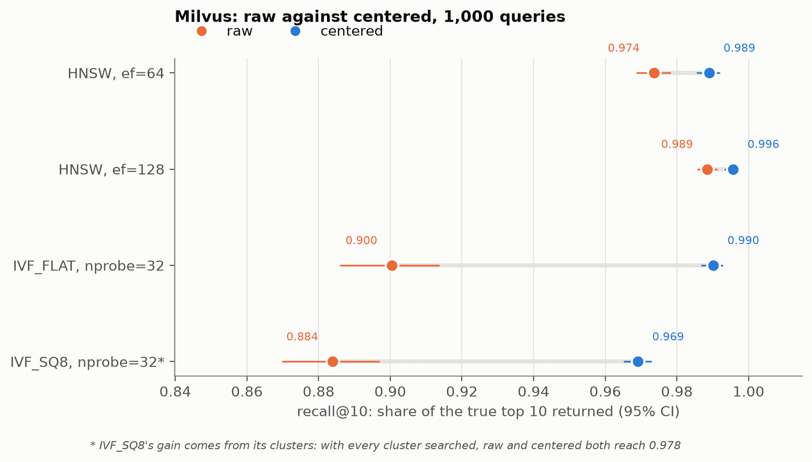Read it like the summary chart in part 1: orange is raw, blue is centered, further right is better, and the gray bar is the gain. The gap is widest on the IVF indexes; on IVF_SQ8 the gain comes from the clusters, not the 8-bit compression.

The correct answer is identical in both columns, so the whole difference comes from the index. HNSW’s graph and IVF’s clusters are both built from the stored vectors. Raw, those vectors are dominated by a height of about 3.23 that barely changes from one image to the next, while the numbers that actually tell images apart are around ±0.02. The index ends up organizing the vectors by the part that doesn’t matter. Centering removes that, and IVF_FLAT goes from missing one true neighbor in ten to missing one in a hundred: ten times fewer misses. HNSW at ef=64 goes from missing 0.026 of the true top 10 to 0.011, less than half as many.

Centered Strategy A with HNSW at ef=128 reaches a recall@10 of 0.996. Strategy B also reaches 0.996 on the same queries. The confidence intervals overlap, so they are effectively equal. A gets B’s recall with one vector and one search: no shortlist, no rerank and no extra fields.

Where centering does not help

Centering fixes how the index organizes the vectors, and it rescues compression that treats all 513 numbers on one scale, such as fp16. It can’t help compression that already handles each number separately, and one index type fails either way.

• IVF_SQ8 at full search (every cluster searched) reaches a recall@10 of about 0.978 raw or centered. Milvus’s vector search engine, Knowhere, uses the 8-bit quantizer from Faiss, an open-source similarity search library. That quantizer (QT_8bit) gives each of the 513 numbers its own value range. The height already gets a range of its own, so centering it changes nothing. A simulated per-number 8-bit codec gives the same recall. (A codec that shared one range across all 513 numbers would be a different story: in simulation, raw vectors fall to a recall of 0.082, and centering lifts them only to 0.642.)
• IVF_PQ (product quantization, which compresses groups of numbers together into short codes) fails either way, and centering makes it slightly worse: recall 0.096 centered against 0.115 raw. Don’t use Strategy A on a PQ index.
• SCANN refuses a 513-dimensional vector outright, because it needs an even number of dimensions.

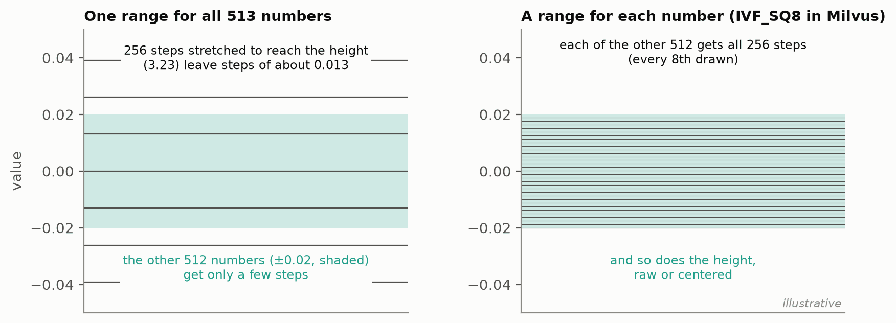Why IVF_SQ8 doesn't need centering. Milvus gives every number its own 8-bit range (right), so the large height can't crowd out the other 512. One range shared by all 513 numbers (left) would.

What we are not claiming

Which configuration is fastest on self-hosted Milvus. Two runs on a laptop, with warm-up, put every single-round-trip configuration at 2 to 3.7 ms, and the two runs disagreed with each other as much as the configurations did. That is too noisy to rank. Part 3 measures latency properly, from a machine in the same cloud region as a Zilliz Cloud cluster.

Exact ImageNet embeddings. For speed, the model ran in fp16 (16-bit floating point) to encode the images, and the hyperbolic geometry was then computed in fp32. That doesn’t affect the recall figures, because the true top 10 is computed exactly (in 64-bit floating point) over whatever vectors are stored.

Takeaway

Hyperbolic search on stock Milvus takes one flipped sign at query time and one subtraction at ingest, with no rerank. On 1.28 million vectors, centered Strategy A reaches a recall@10 of 0.996 on HNSW at ef=128, matching the shortlist-and-rerank design with a single search, and centering lifts IVF_FLAT from 0.900 to 0.990. Use it on HNSW, IVF_FLAT or IVF_SQ8, turning up ef or nprobe for more recall, and avoid IVF_PQ.

Part 3 runs the same vectors on Zilliz Cloud’s managed index, with capacity and latency measured in-region.

---

1. Deng, Jia; Dong, Wei; Socher, Richard; et al. (2009). “ImageNet: A Large-Scale Hierarchical Image Database”. 2009 IEEE Conference on Computer Vision and Pattern Recognition. pp. 248–255. doi:10.1109/CVPR.2009.5206848. ↩

2. Papers and code call this number the time coordinate. The Lorentz model borrows its math from special relativity, where one coordinate is time and the rest are space; nothing here involves time. In this series the name survives only in the field name h_time, in Strategy B below. ↩

3. Madhu, Hiren; Bui, Ngoc; Maatouk, Ali; et al. (2026). “HypRAG: Hyperbolic Dense Retrieval for Retrieval Augmented Generation”. arXiv:2602.07739. ↩