A Day in the Life of a Milvus Datum

Building a performant vector database like Milvus that scales to billions of vectors and handles web-scale traffic is no simple feat. It requires the careful, intelligent design of a distributed system. Necessarily, there will be a trade-off between performance vs simplicity in the internals of a system like this.

While we have tried to well balance this trade-off, some aspects of the internals have remained opaque. This article aims to dispel any mystery around how Milvus breaks down data insertion, indexing, and serving across nodes. Understanding these processes at a high level is essential for effectively optimizing query performance, system stability, and debugging-related issues.

So, let’s take a stroll in a day in the life of Dave, the Milvus datum. Imagine you insert Dave into your collection in a Milvus Distributed deployment (see the diagram below). As far as you are concerned, he goes directly into the collection. Behind the scenes, however, many steps occur across independent sub-systems.

Proxy Nodes and the Message Queue

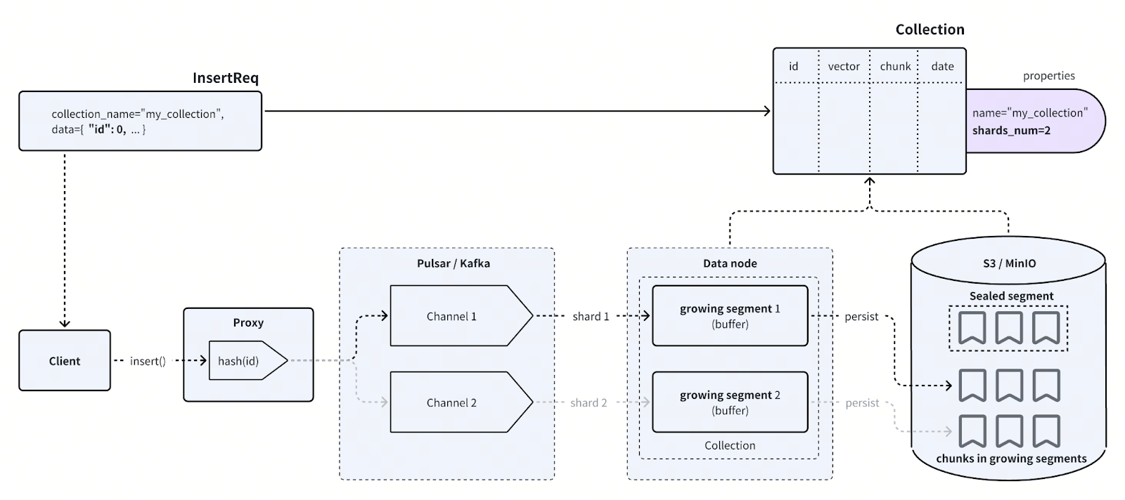
Initially, you call the MilvusClient object, for example, via the PyMilvus library, and send an _insert()_ request to a proxy node. Proxy nodes are the gateway between the user and the database system, performing operations like load balancing on incoming traffic and collating multiple outputs before they are returned to the user.

A hash function is applied to the item’s primary key to determine which channel to send it to. Channels, implemented with either Pulsar or Kafka topics, represent a holding ground for streaming data, which can then be sent onwards to subscribers of the channel.

Data Nodes, Segments, and Chunks

After the data has been sent to the appropriate channel, the channel then sends it to the corresponding segment in the data node. Data nodes are responsible for storing and managing data buffers called growing segments. There is one growing segment per shard.

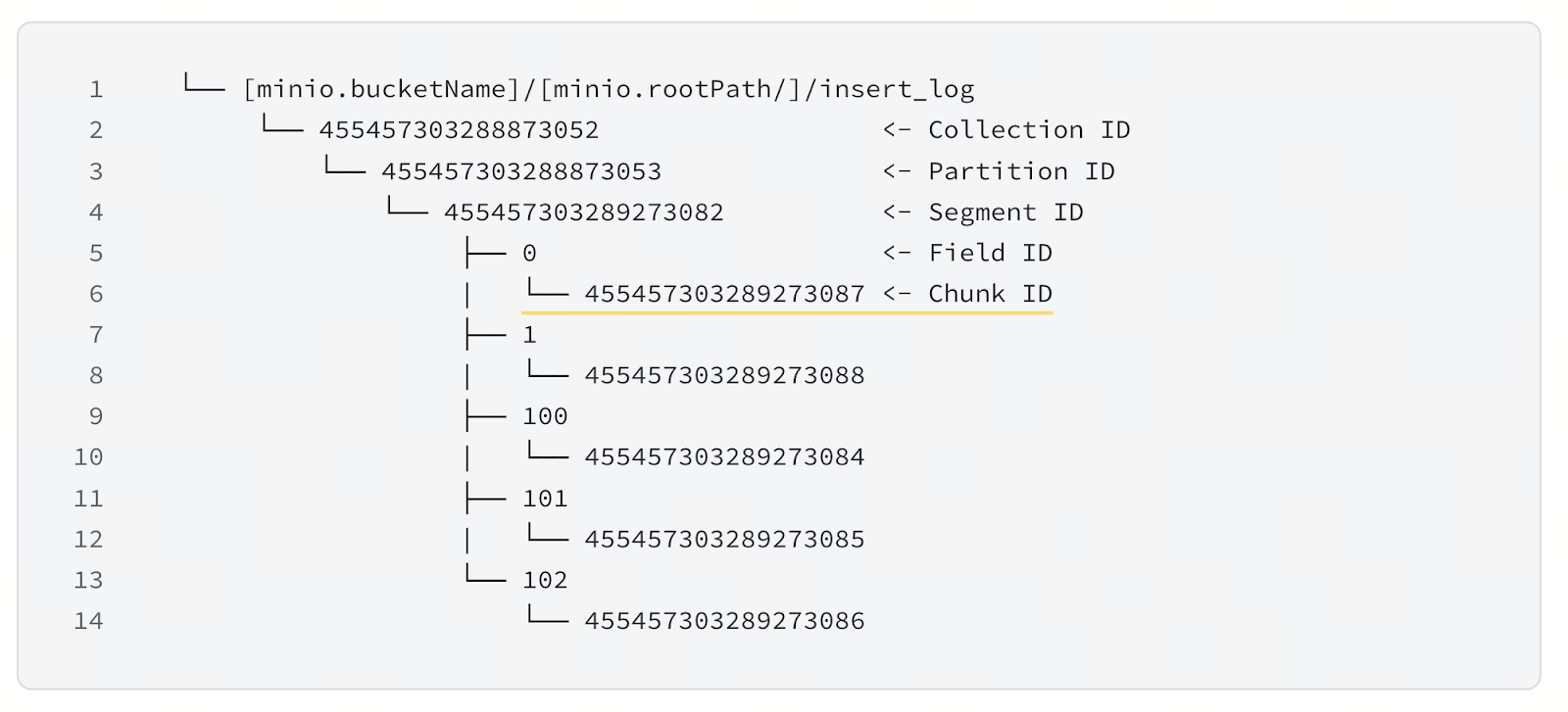
As data is inserted into a segment, the segment grows towards a maximum size, defaulting to 122MB. During this time, smaller parts of the segment, by default 16MB and known as chunks, are pushed to persistent storage, for example, using AWS’s S3 or other compatible storage like MinIO. Each chunk is a physical file on the object storage and there is a separate file per field. See the figure above illustrating the file hierarchy on object storage.

So to summarize, a collection’s data is split across data nodes, within which it is split into segments for buffering, which are further split into per-field chunks for persistent storage. The two diagrams above make this clearer. By dividing the incoming data in this way, we fully exploit the cluster’s parallelism of network bandwidth, compute, and storage.

Sealing, Merging, and Compacting Segments

Thus far we have told the story of how our friendly datum Dave makes his way from an _insert()_ query into persistent storage. Of course, his story does not end there. There are further steps to make the search and indexing process more efficient. By managing the size and number of segments, the system fully exploits the cluster’s parallelism.

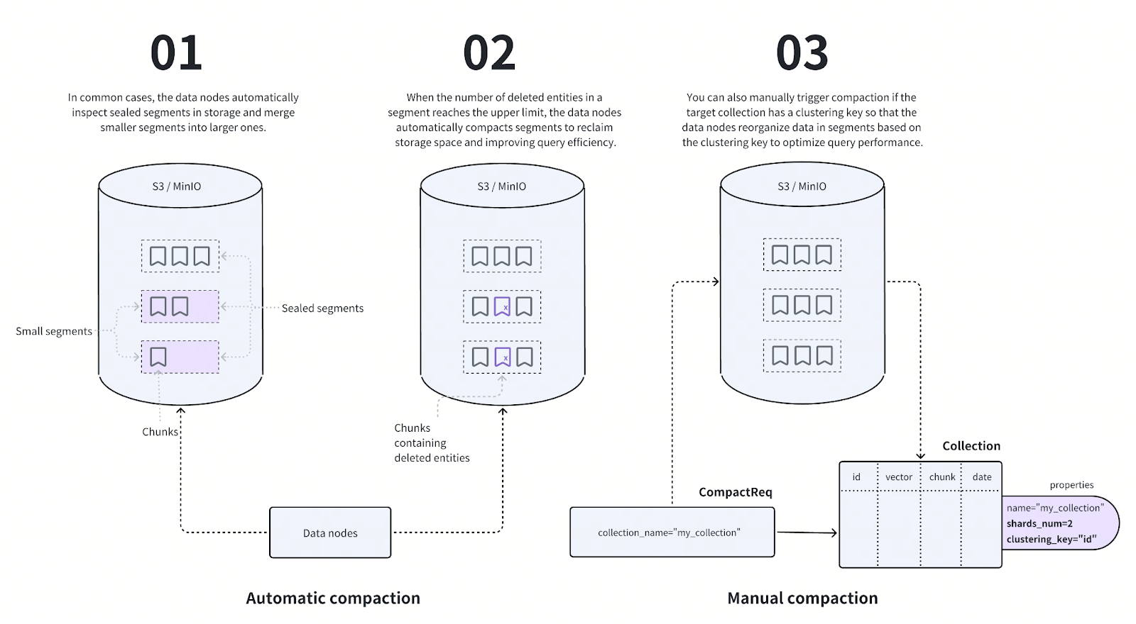
Once a segment reaches its maximum size on a data node, by default 122MB, it is said to be sealed. What this means is that the buffer on the data node is cleared to make way for a new segment, and the corresponding chunks in persistent storage are marked as belonging to a closed segment.

The data nodes periodically look for smaller sealed segments and merge them into larger ones until they have reached a maximum size of 1GB (by default) per segment. Recall that when an item is deleted in Milvus, it is simply marked with a deletion flag - think of it as Death Row for Dave. When the number of deleted items in a segment passes a given threshold, by default 20%, the segment is reduced in size, an operation we call compaction.

Indexing and Searching through Segments

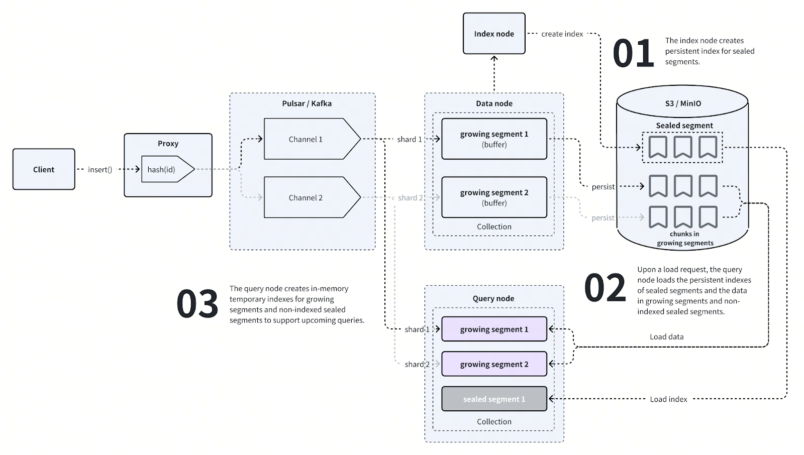
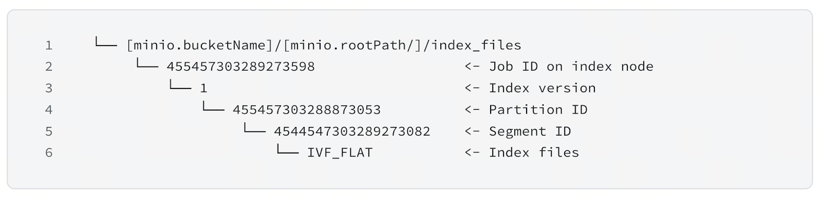
There is an additional node type, the index node, that is responsible for building indexes for sealed segments. When the segment is sealed, the data node sends a request for an index node to construct an index. The index node then sends the completed index to object storage. Each sealed segment has its own index stored in a separate file. You can examine this file manually by accessing the bucket - see the figure above for the file hierarchy.

Query nodes - not only data nodes - subscribe to the message queue topics for the corresponding shards. The growing segments are replicated on the query nodes, and the node loads into memory sealed segments belonging to the collection as required. It builds an index for each growing segment as data comes in, and loads the finalized indexes for sealed segments from the data store.

Imagine now that you call the MilvusClient object with a search() request that encompasses Dave. After being routed to all query nodes via the proxy node, each query node performs a vector similarity search (or another one of the search methods like query, range search, or grouping search), iterating over the segments one by one. The results are collated across nodes in a MapReduce-like fashion and sent back to the user, Dave being happy to find himself reunited with you at last.

Discussion

We have covered a day in the life of Dave the datum, both for _insert()_ and _search()_ operations. Other operations like _delete()_ and _upsert()_ work similarly. Inevitably, we have had to simplify our discussion and omit finer details. On the whole, though, you should now have a sufficient picture of how Milvus is designed for parallelism across nodes in a distributed system to be robust and efficient, and how you can use this for optimization and debugging.

An important takeaway from this article: Milvus is designed with a separation of concerns across node types. Each node type has a specific, mutually exclusive function, and there is a separation of storage and compute. The result is that each component can be scaled independently with parameters tweakable according to the use case and traffic patterns. For example, you can scale the number of query nodes to serve increased traffic without scaling data and index nodes. With that flexibility, there are Milvus users that handle billions of vectors and serve web-scale traffic, with sub-100ms query latency.

You can also enjoy the benefits of Milvus’ distributed design without even deploying a distributed cluster through Zilliz Cloud, a fully managed service of Milvus. Sign up today for the free-tier of Zilliz Cloud and put Dave into action!