

A vector database scales to billions of vectors by combining four ideas: approximate indexes that avoid comparing a query against every vector, compression and tiered storage that shrink how much must sit in RAM, horizontal partitioning that spreads data and work across nodes, and disaggregated architecture that lets ingestion, indexing, and search scale independently. Whether a given system scales for your workload, though, depends less on vector count than on dimension, index type, filters, write rate, and concurrency, all measured at the recall you actually need.
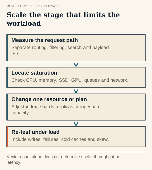 Scale the stage that limits the workload. Vector count alone does not determine useful throughput or latency.
Why is vector count the wrong unit?
“One billion vectors” says little on its own. A billion 768-dimensional float32 vectors is about 3 TB of raw data before any index overhead, while the same count at 128 dimensions is about 0.5 TB. Add an HNSW graph, scalar fields, and JSON metadata and the memory picture changes again. Then serving demand multiplies it: 50 queries per second with top-10 and no filter is a very different load from 5,000 queries per second with a selective metadata filter and top-100.
So describe the workload in full before sizing anything: vector fields and dimensions, data type (float32, float16, int8, binary, sparse), payload size, filter selectivity, top-k, target recall, peak QPS, write and delete rate, and expected growth. The Milvus sizing tool turns those inputs into a starting resource estimate, and estimating memory for vector search explains the arithmetic.
Which architectural features make billion-scale search possible?
Approximate nearest-neighbor indexes. Exact search is linear in corpus size. Graph indexes such as HNSW and cluster indexes such as IVF visit only a small fraction of the data per query, trading a little recall for orders of magnitude less work.
Quantization and disk-based indexes. Scalar quantization, product quantization, and binary codes like RaBitQ shrink vectors several-fold to more than an order of magnitude, and DISKANN keeps most of the index on NVMe while holding a compressed copy in memory. These are the main economic lever at large scale. Vector quantization trade-offs covers how much recall each costs.
Segments. Milvus stores a collection as many segments. New data lands in growing segments, which are sealed, indexed, and compacted in the background. Searches run across segments in parallel and merge the results, so the index never has to be rebuilt as one giant structure.
Sharding and replicas. Writes are spread across shards (each backed by a WAL channel), and sealed segments are distributed across query nodes. In-memory replicas add copies for read throughput and availability. Sharding and replication explains how the two differ.
Disaggregated storage and compute. This is what lets each bottleneck be scaled on its own.
How does Milvus split the work?
Milvus uses a four-layer, fully disaggregated design:
| Layer | Component | What it does | How it scales |
|---|---|---|---|
| Access | Proxy | Stateless entry point; validates requests, fans out, merges results | Add proxies behind a load balancer |
| Coordination | Coordinator | Single active control plane for topology, scheduling, and consistency | Not scaled out (high availability via standby) |
| Workers | Streaming Node | Owns shard WAL consumption and growing data; serves queries on fresh data | Multiple instances |
| Query Node | Loads sealed segments from object storage and searches them | Horizontally, for more data or QPS | |
| Data Node | Background compaction and index building | Horizontally, for ingest-heavy or rebuild workloads | |
| Storage | etcd, object storage (S3, MinIO, Azure Blob), WAL (Woodpecker by default) | Metadata, segments and indexes, durable log | Managed by the storage tier |
Because the durable copy of the data lives in object storage, query nodes are effectively caches you can add or remove, and index building happens on data nodes without stealing CPU from search. Scaling out is a Helm change, for example --set queryNode.replicas=3, and the cluster rebalances segments onto new nodes. When scaling in, the docs advise removing one node at a time. For QPS beyond what one copy can serve, load the collection with more in-memory replicas (replica_number), and use resource groups to give heavy collections their own query nodes. How the Milvus architecture separates ingestion, storage, and search walks through the data path.
How do you find the real bottleneck?
Scalability problems are rarely “the database is too slow” in general. Measure each stage separately: embedding generation, ingestion, segment sealing and index build, load time, search, payload fetch, and reranking. Adding query nodes will not help if the slow step is an external embedding API or a source database. Within Milvus, check which resource saturates first: CPU on query nodes (raise replicas or nodes), memory (quantize, use mmap or DISKANN, or load fewer fields), network on fan-out, or data node backlog during heavy writes. Locating a bottleneck across Milvus components has the metric-by-metric guide.
Filters deserve special attention. A selective filter can make a search cheaper or more expensive depending on how it interacts with the index, and a skewed tenant or partition can become a hotspot while total resources look fine.
How do you prove the next growth step?
A benchmark at one scale does not extrapolate linearly. To show you can grow:
- Pick a fixed recall target and hold it for every comparison, using a FLAT baseline as ground truth.
- Grow data volume, query concurrency, and write traffic one at a time, then together.
- Track p50/p99 latency, error rate, resource utilization, and recall at each step.
- Kill a query node mid-test and measure recovery time and latency during rebalance.
- Include maintenance: compaction, index rebuilds, and bulk loads running alongside traffic.
- Keep headroom, typically enough that one node failure does not breach your SLO.
How to benchmark vector search performance covers tooling and methodology.
When should you split hot and cold data?
At very large scale, not every vector needs the same latency. Recent or popular data can be served from memory while older data sits on cheaper tiers or in a lake, queried less often. Separating hot vector serving from cold lake data describes that pattern.
Next steps
Estimate your deployment with the sizing tool, then validate it with the steps above. If you would rather have elastic scaling handled for you, Zilliz Cloud runs managed Milvus; compare current pricing against the costs of managed and self-hosted vector search.


