Home
Blog
Smarter Retrieval for RAG: Late Chunking with Jina Embeddings v2 and Milvus

Smarter Retrieval for RAG: Late Chunking with Jina Embeddings v2 and Milvus

Tutorials

October 11, 2025

Wei Zang

Building a robust RAG system usually starts with document chunking—splitting large texts into manageable pieces for embedding and retrieval. Common strategies include:

Fixed‑size chunks (e.g., every 512 tokens)
Variable‑size chunks (e.g., paragraph or sentence boundaries)
Sliding windows (overlapping spans)
Recursive chunking (hierarchical splits)
Semantic chunking (grouping by topic)

While these methods have their merits, they often fracture long‑range context. To address this challenge, Jina AI creates a Late Chunking approach: embed the entire document first, then carve out your chunks.

In this article, we’ll explore how Late Chunking works and demonstrate how combining it with Milvus—a high-performance open-source vector database built for similarity search—can dramatically improve your RAG pipelines. Whether you’re building enterprise knowledge bases, AI-driven customer support, or advanced search applications, this walkthrough will show you how to manage embeddings more effectively at scale.

What Is Late Chunking?

Traditional chunking methods can break important connections when key information spans multiple chunks—resulting in poor retrieval performance.

Consider these release notes for Milvus 2.4.13, split into two chunks like below:

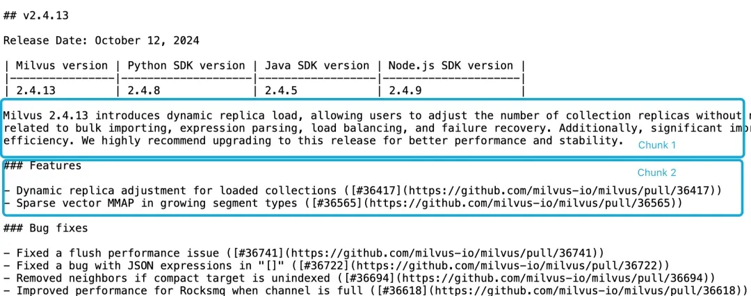
Figure 1. Chunking Milvus 2.4.13 Release Note

If you query, “What are the new features in Milvus 2.4.13?”, a standard embedding model may fail to link “Milvus 2.4.13” (in Chunk 1) with its features (in Chunk 2). The result? Weaker vectors and lower retrieval accuracy.

Heuristic fixes—such as sliding windows, overlapping contexts, and repeated scans—provide partial relief but no guarantees.

Traditional chunking follows this pipeline:

Pre‑chunk text (by sentences, paragraphs, or max token length).
Embed each chunk separately.
Aggregate token embeddings (e.g., via average pooling) into a single chunk vector.

Late Chunking flips the pipeline:

Embed first: Run a long‑context transformer over the full document, generating rich token embeddings that capture global context.
Chunk later: Average‑pool contiguous spans of those token embeddings to form your final chunk vectors.

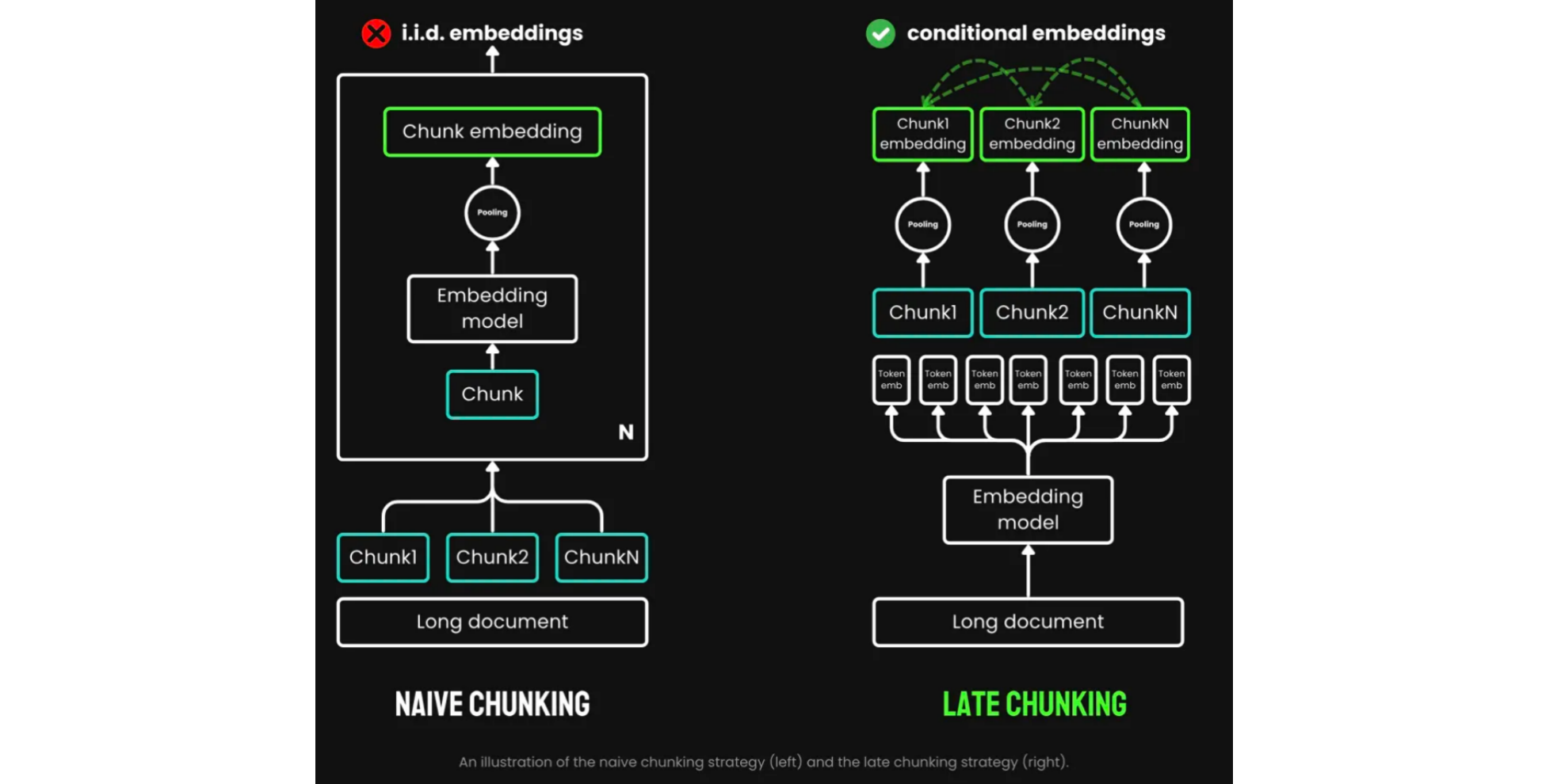
Figure 2. Naive Chunking vs. Late Chunking (Source)

By preserving full‑document context in every chunk, Late Chunking yields:

Higher retrieval accuracy—each chunk is contextually aware.
Fewer chunks—you send more focused text to your LLM, cutting costs and latency.

Many long‑context models like jina-embeddings-v2-base-en can process up to 8,192 tokens—equivalent to about a 20-minute read (roughly 5,000 words)—making Late Chunking practical for most real‑world documents.

Now that we understand the “what” and “why” behind Late Chunking, let’s dive into the “how”. In the next section, we’ll guide you through a hands‑on implementation of the Late Chunking pipeline, benchmark its performance against traditional chunking, and validate its real‑world impact using Milvus. This practical walkthrough will bridge theory and practice, showing exactly how to integrate Late Chunking into your RAG workflows.

Testing Late Chunking

Basic Implementation

Below are the core functions for Late Chunking. We’ve added clear docstrings to guide you through each step. The function sentence_chunker splits the original document into paragraph‑based chunks, returning both the chunk contents and the chunk annotation information span_annotations (i.e., the start and end indices of each chunk).

def sentence_chunker(document, batch_size=10000):
    nlp = spacy.blank("en")
    nlp.add_pipe("sentencizer", config={"punct_chars": None})
    doc = nlp(document)

    docs = []
    for i in range(0, len(document), batch_size):
        batch = document[i : i + batch_size]
        docs.append(nlp(batch))

    doc = Doc.from_docs(docs)

    span_annotations = []
    chunks = []
    for i, sent in enumerate(doc.sents):
        span_annotations.append((sent.start, sent.end))
        chunks.append(sent.text)

    return chunks, span_annotations

The function document_to_token_embeddings uses the jinaai/jina-embeddings-v2-base-en model and its tokenizer to produce embeddings for the entire document.

def document_to_token_embeddings(model, tokenizer, document, batch_size=4096):
    tokenized_document = tokenizer(document, return_tensors="pt")
    tokens = tokenized_document.tokens()

    outputs = []
    for i in range(0, len(tokens), batch_size):
        
        start = i
        end   = min(i + batch_size, len(tokens))

        batch_inputs = {k: v[:, start:end] for k, v in tokenized_document.items()}

        with torch.no_grad():
            model_output = model(**batch_inputs)

        outputs.append(model_output.last_hidden_state)

    model_output = torch.cat(outputs, dim=1)
    return model_output

The function late_chunking takes the document’s token embeddings and the original chunk annotation information span_annotations, and then produces the final chunk embeddings.

def late_chunking(token_embeddings, span_annotation, max_length=None):
    outputs = []
    for embeddings, annotations in zip(token_embeddings, span_annotation):
        if (
            max_length is not None
        ):
            annotations = [
                (start, min(end, max_length - 1))
                for (start, end) in annotations
                if start < (max_length - 1)
            ]
        pooled_embeddings = []
        for start, end in annotations:
            if (end - start) >= 1:
                pooled_embeddings.append(
                    embeddings[start:end].sum(dim=0) / (end - start)
                )
                    
        pooled_embeddings = [
            embedding.detach().cpu().numpy() for embedding in pooled_embeddings
        ]
        outputs.append(pooled_embeddings)

    return outputs

For example, chunking with jinaai/jina-embeddings-v2-base-en:

tokenizer = AutoTokenizer.from_pretrained('jinaai/jina-embeddings-v2-base-en', trust_remote_code=True)
model     = AutoModel.from_pretrained('jinaai/jina-embeddings-v2-base-en', trust_remote_code=True)

# First chunk the text as normal, to obtain the beginning and end points of the chunks.
chunks, span_annotations = sentence_chunker(document)
# Then embed the full document.
token_embeddings = document_to_token_embeddings(model, tokenizer, document)
# Then perform the late chunking
chunk_embeddings = late_chunking(token_embeddings, [span_annotations])[0]

Tip: Wrapping your pipeline in functions makes it easy to swap in other long‑context models or chunking strategies.

Comparison with Traditional Embedding Methods

To further demonstrate the advantages of Late Chunking, we also compared it to traditional embedding approaches, using a set of sample documents and queries.

And let’s revisit our Milvus 2.4.13 release note example:

Milvus 2.4.13 introduces dynamic replica load, allowing users to adjust the number of collection replicas without needing to release and reload the collection. This version also addresses several critical bugs related to bulk importing, expression parsing, load balancing, and failure recovery. Additionally, significant improvements have been made to MMAP resource usage and import performance, enhancing overall system efficiency. We highly recommend upgrading to this release for better performance and stability.

We measure cosine similarity between the query embedding (“milvus 2.4.13”) and each chunk:

cos_sim = lambda x, y: np.dot(x, y) / (np.linalg.norm(x) * np.linalg.norm(y))

milvus_embedding = model.encode('milvus 2.4.13')

for chunk, late_chunking_embedding, traditional_embedding in zip(chunks, chunk_embeddings, embeddings_traditional_chunking):
    print(f'similarity_late_chunking("milvus 2.4.13", "{chunk}")')
    print('late_chunking: ', cos_sim(milvus_embedding, late_chunking_embedding))
    print(f'similarity_traditional("milvus 2.4.13", "{chunk}")')
    print('traditional_chunking: ', cos_sim(milvus_embedding, traditional_embeddings))

Late Chunking consistently outperformed traditional chunking, yielding higher cosine similarities across every chunk. This confirms that embedding the full document first preserves global context more effectively.

similarity_late_chunking("milvus 2.4.13", "Milvus 2.4.13 introduces dynamic replica load, allowing users to adjust the number of collection replicas without needing to release and reload the collection.")
late_chunking: 0.8785206
similarity_traditional("milvus 2.4.13", "Milvus 2.4.13 introduces dynamic replica load, allowing users to adjust the number of collection replicas without needing to release and reload the collection.")
traditional_chunking: 0.8354263

similarity_late_chunking("milvus 2.4.13", "This version also addresses several critical bugs related to bulk importing, expression parsing, load balancing, and failure recovery.")
late_chunking: 0.84828955
similarity_traditional("milvus 2.4.13", "This version also addresses several critical bugs related to bulk importing, expression parsing, load balancing, and failure recovery.")
traditional_chunking: 0.7222632

similarity_late_chunking("milvus 2.4.13", "Additionally, significant improvements have been made to MMAP resource usage and import performance, enhancing overall system efficiency.")
late_chunking: 0.84942204
similarity_traditional("milvus 2.4.13", "Additionally, significant improvements have been made to MMAP resource usage and import performance, enhancing overall system efficiency.")
traditional_chunking: 0.6907381

similarity_late_chunking("milvus 2.4.13", "We highly recommend upgrading to this release for better performance and stability.")
late_chunking: 0.85431844
similarity_traditional("milvus 2.4.13", "We highly recommend upgrading to this release for better performance and stability.")
traditional_chunking: 0.71859795

We can see that embedding the full paragraph first ensures each chunk carries the “Milvus 2.4.13” context—boosting similarity scores and retrieval quality.

Testing Late Chunking in Milvus

Once chunk embeddings are generated, we can store them in Milvus and perform queries. The following code inserts chunk vectors into the collection.

Importing Embeddings into Milvus

batch_data=[]
for i in range(len(chunks)):
    data = {
            "content": chunks[i],
            "embedding": chunk_embeddings[i].tolist(),
        }

    batch_data.append(data)

res = client.insert(
    collection_name=collection,
    data=batch_data,
)

Querying and Validation

To validate the accuracy of Milvus queries, we compare its retrieval results to brute-force cosine similarity scores calculated manually. If both methods return consistent top‑k results, we can be confident that Milvus’s search accuracy is reliable.

We compare Milvus’s native search with a brute‑force cosine similarity scan:

def late_chunking_query_by_milvus(query, top_k = 3):
    query_vector = model(**tokenizer(query, return_tensors="pt")).last_hidden_state.mean(1).detach().cpu().numpy().flatten()

    res = client.search(
                collection_name=collection,
                data=[query_vector.tolist()],
                limit=top_k,
                output_fields=["id", "content"],
            )

    return [item.get("entity").get("content") for items in res for item in items]

def late_chunking_query_by_cosine_sim(query, k = 3):
    cos_sim = lambda x, y: np.dot(x, y) / (np.linalg.norm(x) * np.linalg.norm(y))
    query_vector = model(**tokenizer(query, return_tensors="pt")).last_hidden_state.mean(1).detach().cpu().numpy().flatten()

    results = np.empty(len(chunk_embeddings))
    for i, (chunk, embedding) in enumerate(zip(chunks, chunk_embeddings)):
        results[i] = cos_sim(query_vector, embedding)

    results_order = results.argsort()[::-1]
    return np.array(chunks)[results_order].tolist()[:k]

This confirms Milvus returns the same top‑k chunks as a manual cosine‑sim scan.

> late_chunking_query_by_milvus("What are new features in milvus 2.4.13", 3)

['\n\n### Features\n\n- Dynamic replica adjustment for loaded collections ([#36417](https://github.com/milvus-io/milvus/pull/36417))\n- Sparse vector MMAP in growing segment types ([#36565](https://github.com/milvus-io/milvus/pull/36565))...

> late_chunking_query_by_cosine_sim("What are new features in milvus 2.4.13", 3)

['\n\n### Features\n\n- Dynamic replica adjustment for loaded collections ([#36417](https://github.com/milvus-io/milvus/pull/36417))\n- Sparse vector MMAP in growing segment types (#36565)...

So both methods yield the same top-3 chunks, confirming Milvus’s accuracy.

Conclusion

In this article, we took a deep dive into the mechanics and benefits of Late Chunking. We began by identifying the shortcomings of traditional chunking approaches, particularly when handling long documents where preserving context is crucial. We introduced the concept of Late Chunking—embedding the entire document before slicing it into meaningful chunks—and showed how this preserves global context, leading to improved semantic similarity and retrieval accuracy.

We then walked through a hands-on implementation using Jina AI’s jina-embeddings-v2-base-en model and evaluated its performance compared to traditional methods. Finally, we demonstrated how to integrate the chunk embeddings into Milvus for scalable and accurate vector search.

Late Chunking offers a context‑first approach to embedding—perfect for long, complex documents where context matters most. By embedding the entire text upfront and slicing later, you gain: