Managing Data in Massive-Scale Vector Search Engine
Author: Yihua Mo
Date: 2019-11-08
How data management is done in Milvus
First of all, some basic concepts of Milvus:
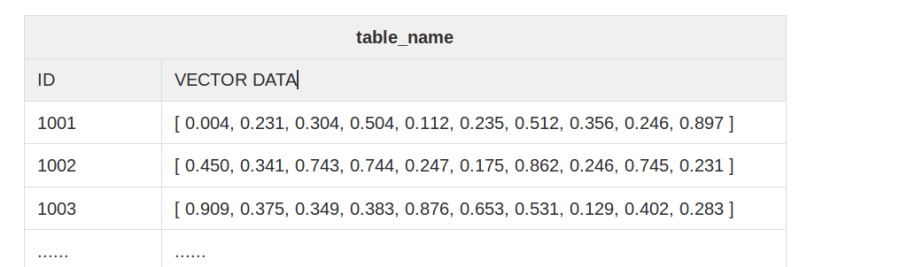
- Table: Table is a data set of vectors, with each vector having a unique ID. Each vector and its ID represent a row of the table. All vectors in a table must have the same dimensions. Below is an example of a table with 10-dimensional vectors:
 table
table
- Index: Building index is the process of vector clustering by certain algorithm, which requires additional disk space. Some index types require less space since they simplify and compress vectors, while some other types require more space than raw vectors.
In Milvus, users can perform tasks such as creating a table, inserting vectors, building indexes, searching vectors, retrieving table information, dropping tables, removing partial data in a table and removing indexes, etc.
Assume we have 100 million 512-dimensional vectors, and need to insert and manage them in Milvus for efficient vector search.
(1) Vector Insert
Let’s take a look at how vectors are inserted into Milvus.
As each vector takes 2 KB space, the minimum storage space for 100 million vectors is about 200 GB, which makes one-time insertion of all these vectors unrealistic. There need to be multiple data files instead of one. Insertion performance is one of the key performance indicators. Milvus supports one-time insertion of hundreds or even tens of thousands of vectors. For example, one-time insertion of 30 thousand 512-dimensional vectors generally takes only 1 second.
 insert
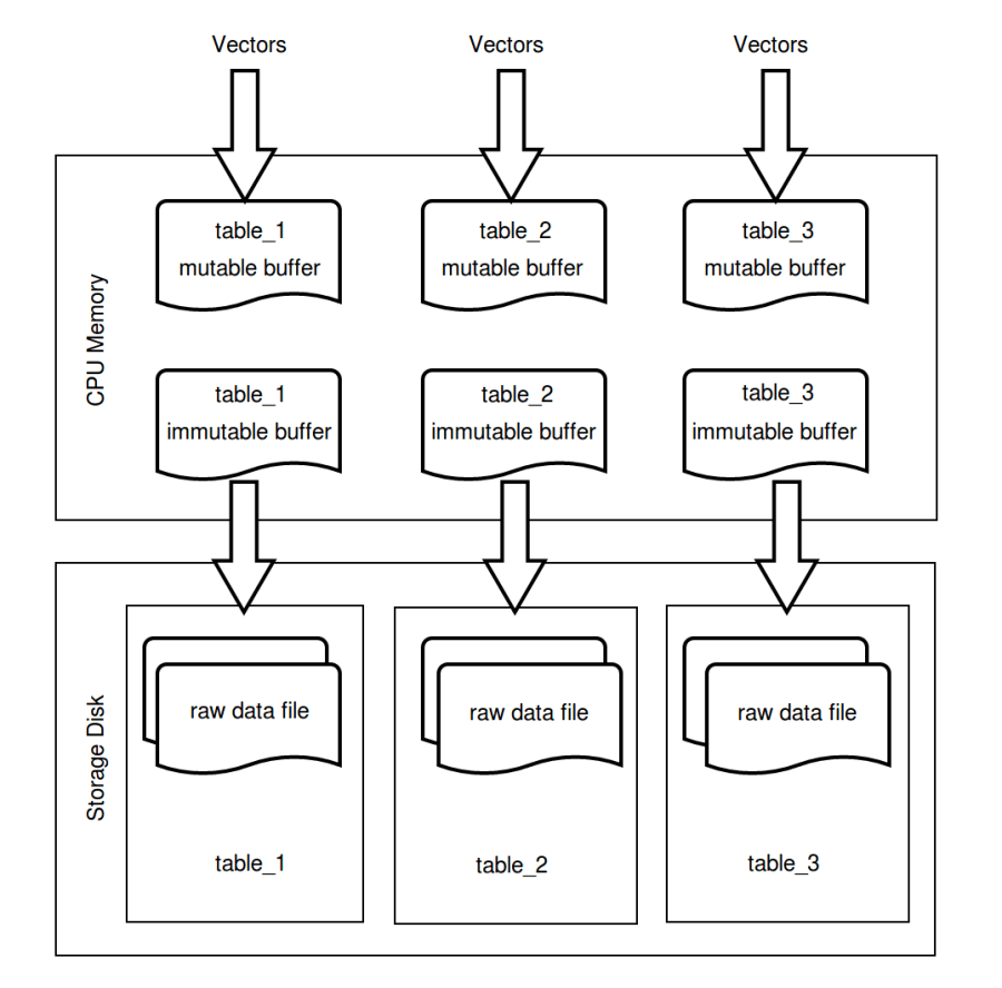
Not every vector insertion is loaded into disk. Milvus reserves a mutable buffer in the CPU memory for every table that is created, where inserted data can be quickly written to. And as the data in the mutable buffer reaches a certain size, this space will be labeled as immutable. In the mean time, a new mutable buffer will be reserved. Data in immutable buffer are written to disk regularly and corresponding CPU memory is freed up. The regular writing to disk mechanism is similar to the one used in Elasticsearch, which writes buffered data to disk every 1 second. In addition, users that are familiar with LevelDB/RocksDB can see some resemblance to MemTable here.
The goals of the Data Insert mechanism are:
- Data insertion must be efficient.
- Inserted data can be used instantly.
- Data files should not be too fragmented.
(2) Raw Data File
When vectors are written to disk, they are saved in Raw Data File containing the raw vectors. As mentioned before, massive-scale vectors need to be saved and managed in multiple data files. Inserted data size varies as users can insert 10 vectors, or 1 million vectors at one time. However, the operation of writing to disk is executed once every 1 second. Thus data files of different sizes are generated.
Fragmented data files are neither convenient to manage nor easy to access for vector search. Milvus constantly merges these small data files until the merged file size reaches a particular size, for example, 1GB. This particular size can be configured in the API parameter index_file_size in table creation. Therefore, 100 million 512-dimensional vectors will be distributed and saved in about 200 data files.
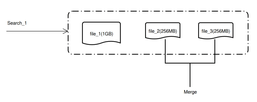
In consideration to incremental computation scenarios, where vectors are inserted and searched concurrently, we need to make sure that once vectors are written to disk, they are available for search. Thus, before the small data files are merged, they can be accessed and searched. Once the merge is completed, the small data files will be removed, and newly merged files will be used for search instead.
This is how queried files look before the merge:
 rawdata1
Queried files after the merge:
 rawdata2
(3) Index File
The search based on Raw Data File is brute-force search which compares the distances between query vectors and origin vectors, and computes the nearest k vectors. Brute-force search is inefficient. Search efficiency can be greatly increased if the search is based on Index File where vectors are indexed. Building index requires additional disk space and is usually time-consuming.
So what are the differences between Raw Data Files and Index Files? To put it simple, Raw Data File records every single vector together with their unique ID while Index File records vector clustering results such as index type, cluster centroids, and vectors in each cluster.
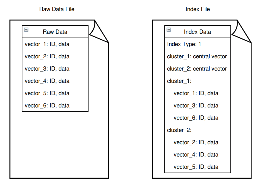 indexfile
Generally speaking, Index File contains more information than Raw Data File, yet the file sizes are much smaller as vectors are simplified and quantized during the index building process (for certain index types).
Newly created tables are by default searched by brute-computation. Once the index is created in the system, Milvus will automatically build index for merged files that reach the size of 1 GB in a standalone thread. When the index building is completed, a new Index File is generated. The raw data files will be archived for index building based on other index types.
Milvus automatically build index for files that reach 1 GB:
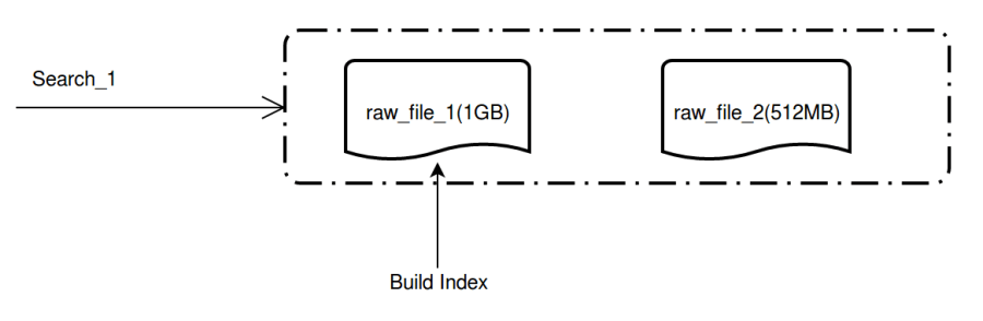 buildindex
Index building completed:
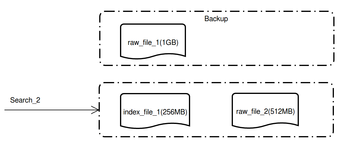 indexcomplete
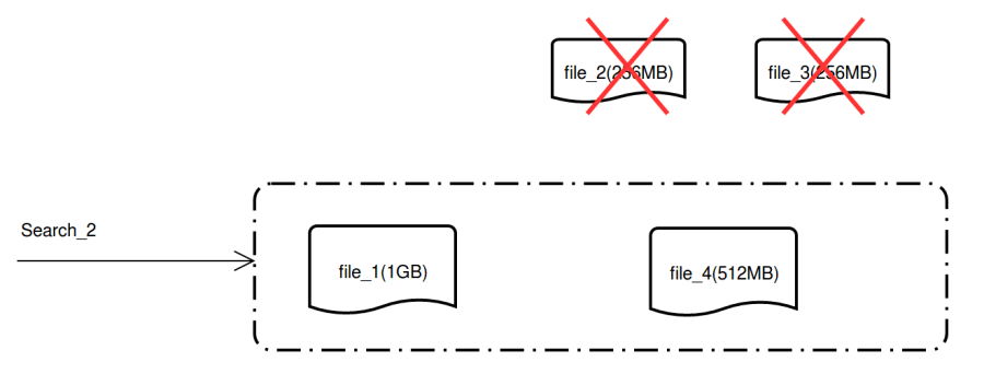
Index will not be automatically built for raw data files that do not reach 1 GB, which may slow down the search speed. To avoid this situation, you need to manually force build index for this table.
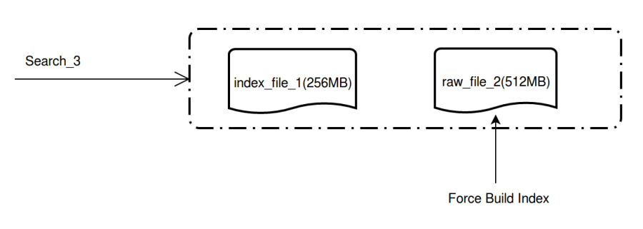 forcebuild
After index is force built for the file, the search performance is greatly enhanced.
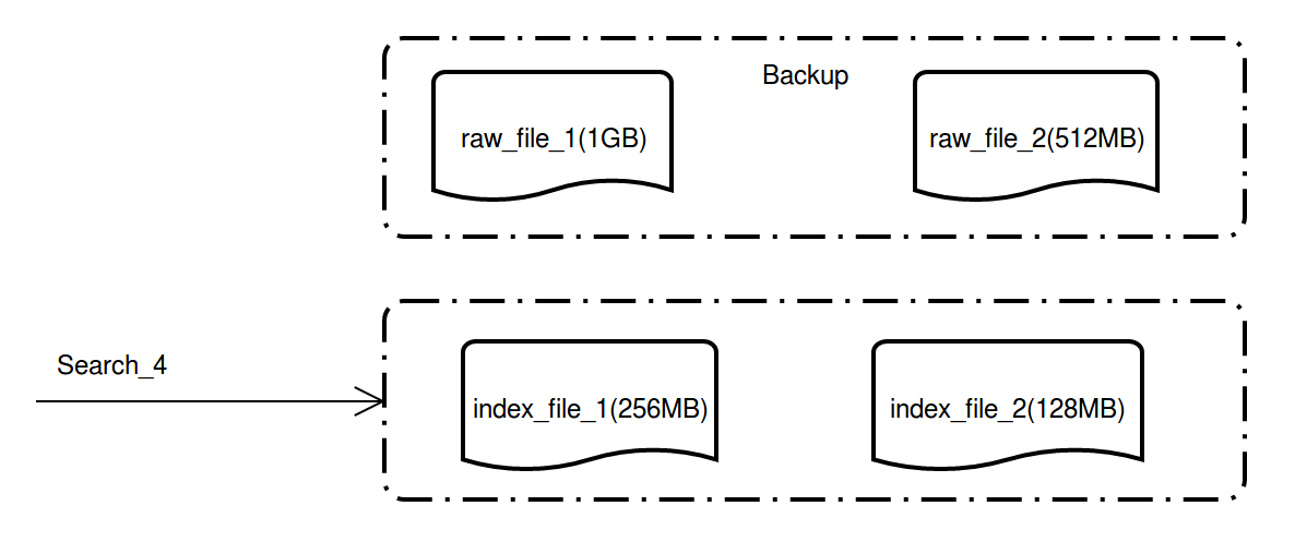 indexfinal
(4) Meta Data
As mentioned earlier, 100 million 512-dimensional vectors are saved in 200 disk files. When index is built for these vectors, there would be 200 additional index files, which makes the total number of files to 400 (including both disk files and index files). An efficient mechanism is required to manage the meta data (file statuses and other information) of these files in order to check the file statuses, remove or create files.
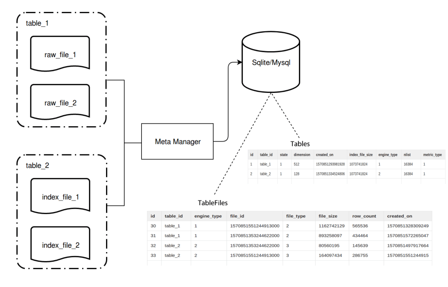
Using OLTP databases to manage these information is a good choice. Standalone Milvus uses SQLite to manage meta data while in distributed deployment, Milvus uses MySQL. When Milvus server starts, 2 tables (namely ‘Tables’ and ‘TableFiles’) are created in SQLite/MySQL respectively. ‘Tables’ records table information and ‘TableFiles’ records information of data files and index files.
As demonstrated in below flowchart, ‘Tables’ contains meta data information such as table name (table_id), vector dimension (dimension), table creation date (created_on), table status (state), index type (engine_type), and number of vector clusters (nlist) and distance computation method (metric_type).
And ‘TableFiles’ contains name of the table the file belongs to (table_id), index type of the file (engine_type), file name (file_id), file type (file_type), file size (file_size), number of rows (row_count) and file creation date (created_on).
 metadata
With these meta data, various operations can be executed. The following are some examples:
- To create a table, Meta Manager only needs to execute a SQL statement:
INSERT INTO TABLES VALUES(1, 'table_2, 512, xxx, xxx, ...). - To execute vector search on table_2, Meta Manager will execute a query in SQLite/MySQL, which is a de facto SQL statement:
SELECT * FROM TableFiles WHERE table_id='table_2'to retrieve the file information of table_2. Then these files will be loaded into memory by Query Scheduler for search computation. - It is not allowed to instantly delete a table as there might be queries being executed on it. That’s why there are soft-delete and hard-delete for a table. When you delete a table, it will be labeled as ‘soft-delete’, and no further querying or changes are allowed to be made to it. However, the queries that were running before the deletion is still going on. Only when all these pre-deletion queries are completed, the table, together with its meta data and related files, will be hard-deleted for good.
(5) Query Scheduler
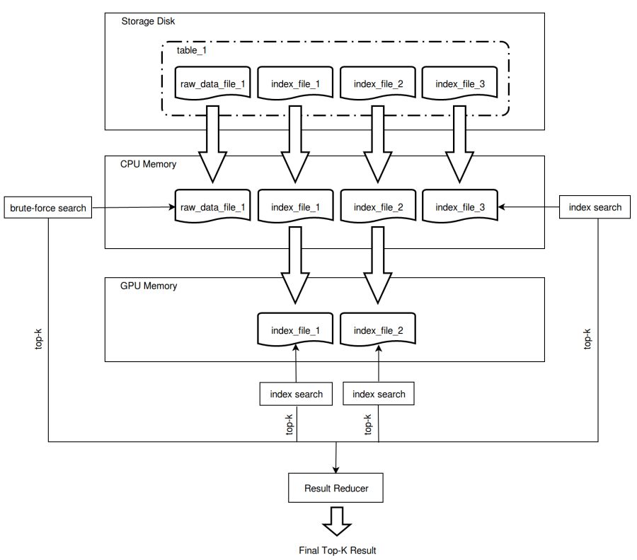
Below chart demonstrates the vector search process in both CPU and GPU by querying files (raw data files and index files) which are copied and saved in disk, CPU memory and GPU memory for the topk most similar vectors.
 topkresult
Query scheduling algorithm significantly improves system performance. The basic design philosophy is to achieve the best search performance through maximum utilization of hardware resources. Below is just a brief description of query scheduler and there will be a dedicated article about this topic in the future.
We call the first query against a given table the ‘cold’ query, and subsequent queries the ‘warm’ query. When the first query is made against a given table, Milvus does a lot of work to load data into CPU memory, and some data into GPU memory, which is time-consuming. In further queries, the search is much faster as partial or all the data are already in CPU memory which saves the time to read from the disk.
To shorten the search time of the first query, Milvus provides Preload Table (preload_table) configuration which enables automatic pre-loading of tables into CPU memory upon server start-up. For a table containing 100 million 512-dimensional vectors, which is 200 GB, the search speed is the fastest if there’s enough CPU memory to store all these data. However, if the table contains billion-scale vectors, it is sometimes inevitable to free up CPU/GPU memory to add new data that are not queried. Currently, we use LRU (Latest Recently Used) as the data replacement strategy.
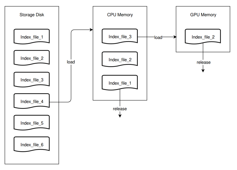
As shown in below chart, assume there is a table that has 6 index files stored on the disk. The CPU memory can only store 3 index files, and GPU memory only 1 index file.
When the search starts, 3 index files are loaded into CPU memory for query. The first file will be released from CPU memory immediately after it is queried. Meanwhile, the 4th file is loaded into CPU memory. In the same way, when a file is queried in GPU memory, it will be instantly released and replaced with a new file.
Query scheduler mainly handles 2 sets of task queues, one queue is about data loading and another is about search execution.
 queryschedule
(6) Result Reducer
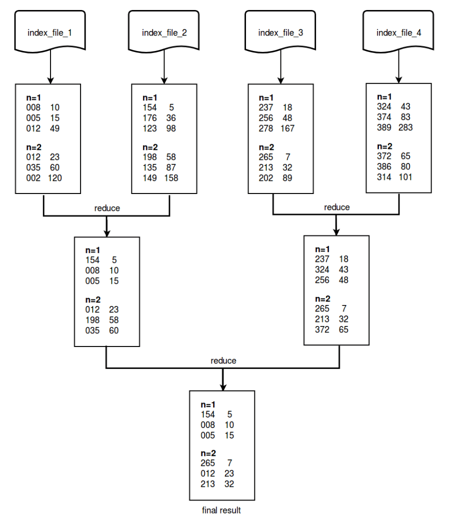
There are 2 key parameters related to vector search: one is ’n’ which means n number of target vectors; another is ‘k’ meaning the top k most similar vectors. The search results are actually n sets of KVP (key-value pairs), each having k pairs of key-value. As queries need to be executed against each individual file, no matter it is raw data file or index file, n sets of top-k result sets will be retrieved for each file. All these result sets are merged to get the top-k result sets of the table.
Below example shows how result sets are merged and reduced for the vector search against a table with 4 index files (n=2, k=3). Note that each result set has 2 columns. The left column represents the vector id and the right column represents the Euclidean distance.
 result
(7) Future Optimization
The following are some thoughts on possible optimizations of data management.
- What if the data in immutable buffer or even mutable buffer can also be instantly queried? Currently, the data in immutable buffer cannot be queried, not until they are written to disk. Some users are more interested in instantaneous access of data after insertion.
- Provide table partitioning functionality that allows user to divide very large tables into smaller partitions, and execute vector search against a given partition.
- Add to vectors some attributes which can be filtered. For example, some users only want to search among the vectors with certain attributes. It is required to retrieve vector attributes and even raw vectors. One possible approach is to use a KV database such as RocksDB.
- Provide data migration functionality that enables automatic migration of outdated data to other storage space. For some scenarios where data flows in all the time, data might be aging. As some users only care about and execute searches against the data of the most recent month, the older data become less useful yet they consume much disk space. A data migration mechanism helps free up disk space for new data.
Summary
This article mainly introduces the data management strategy in Milvus. More articles about Milvus distributed deployment, selection of vector indexing methods and query scheduler will be coming soon. Stay tuned!
Related blogs
Try Managed Milvus for Free
Zilliz Cloud is hassle-free, powered by Milvus and 10x faster.
Get StartedLike the article? Spread the word