

Approximate nearest-neighbor (ANN) search finds vectors that are very close to a query vector without comparing the query against every vector in the collection. It uses an index (a graph, a set of clusters, hash buckets, or compressed codes) to examine only a small, promising fraction of the data, and in exchange it may occasionally miss one of the true closest neighbors. That trade of a little accuracy for orders-of-magnitude less work is what makes semantic search, RAG, and recommendation practical over millions or billions of embeddings.
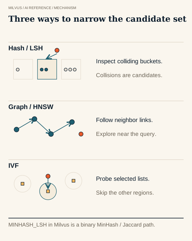 Hash buckets, graph navigation, and IVF partitions are different ANN structures
What problem does nearest-neighbor search solve?
Every nearest-neighbor query has four inputs: a query vector, the set of vectors that are eligible to be returned (after any filters), a distance metric, and a result count k. The task is to return the k stored vectors closest to the query under that metric. This is the k-nearest-neighbor (kNN) problem.
The metric defines what “close” means. Text and image embeddings are usually compared with cosine similarity or inner product, while some models are trained for Euclidean (L2) distance; binary fingerprints use Hamming or Jaccard. The same index can give very different results if the metric does not match how the embedding model was trained, so the metric is part of the question, not a tuning knob. See how cosine, inner product, and L2 differ.
Exact kNN vs ANN: what is the difference?
| Exact kNN (brute force) | Approximate NN | |
|---|---|---|
| How it searches | Computes the distance to every eligible vector | Uses an index to visit a small subset of candidates |
| Result guarantee | The true top-k for the metric | Most of the true top-k, measured as recall |
| Query cost | Grows linearly: roughly N × d operations per query | Typically sublinear in N, tunable per query |
| Extra memory | None beyond the vectors | Graph links, centroids, codebooks, or hash tables |
| Build step | None | Training and/or graph construction |
Exact search is simple and always correct, and for a few thousand vectors it is fast enough. The problem is scale: one million 768-dimensional vectors means about 768 million multiply-adds for a single query, and a busy service runs thousands of queries per second. ANN indexes cut that to a few thousand distance computations by deciding early which regions of the space can be ignored.
Formally, a c-approximate method may return a point whose distance is at most c times the distance to the true nearest neighbor. In practice, vector databases describe approximation with Recall@k: the fraction of the true top-k neighbors (computed with exact search) that the ANN result contains, averaged over a query set. A recall of 0.95 at k=10 means that on average 9.5 of the 10 exact neighbors were returned.
Why can’t classic indexes like k-d trees solve this?
Tree structures such as k-d trees and R-trees work well in two or three dimensions because each split eliminates half the space. Embeddings have hundreds or thousands of dimensions, and in that regime distances between random points concentrate: the nearest and farthest points are almost the same distance away, and a query’s neighborhood touches so many tree cells that the search degrades toward a full scan. This is the curse of dimensionality, and it is why practical high-dimensional search gave up on exact guarantees and moved to approximate structures.
How do ANN algorithms work?
Almost every ANN index combines two ideas: a way to select candidates and a way to represent vectors cheaply enough to score them.
Hashing (LSH). Locality-sensitive hash functions are designed so that similar vectors are likely to land in the same bucket. A query is hashed, and only vectors in matching buckets are compared. LSH has clean theory but usually needs many hash tables to reach high recall on dense embeddings. Its strongest modern use is near-duplicate detection on set similarity, which is what Milvus MINHASH_LSH does for binary MinHash signatures under Jaccard similarity (how MINHASH_LSH finds near-duplicates).
Trees. Space-partitioning trees (k-d trees, random projection forests such as Annoy) split the space recursively. They are easy to reason about but lose efficiency as dimensionality grows, so they are rarely the main index in vector databases today.
Clustering / inverted files (IVF). k-means divides the vectors into nlist clusters. At query time, the search compares the query with the cluster centroids, then scans only the nprobe closest clusters. Fewer probes mean faster queries and a higher chance that a true neighbor sat in an unvisited cluster. How IVF uses centroids walks through this step by step.
Proximity graphs. Each vector becomes a node linked to some of its neighbors. A search starts at an entry point and greedily moves to whichever neighbor is closer to the query, keeping a candidate list until it stops improving. HNSW adds a hierarchy of sparse upper layers for long jumps, giving roughly logarithmic search cost; DiskANN’s Vamana graph is laid out for SSD reads; CAGRA is built for GPU parallelism. Graphs usually give the best recall-per-millisecond in memory, at the cost of storing the links. See what HNSW is and how to tune it.
Quantization. Instead of choosing candidates, quantization shrinks each vector: scalar quantization stores each coordinate in fewer bits, product quantization (PQ) replaces sub-vectors with codebook IDs, and RaBitQ reduces vectors to about one bit per dimension with an error bound. Quantization is usually layered on top of IVF or a graph (IVF_PQ, HNSW_SQ), and a refinement step can rescore top candidates with higher-precision vectors. The vector quantization guide covers the memory arithmetic.
What trade-offs should you expect?
ANN tuning is a triangle between recall, latency (or throughput), and memory, with build time as a fourth corner. Search-time knobs such as ef for HNSW or nprobe for IVF move you along a recall-latency curve for a fixed index; build-time choices such as graph degree, cluster count, or quantization level change the curve itself and its memory footprint. Benchmarks such as ANN-Benchmarks report results as recall-versus-queries-per-second curves for exactly this reason: a single speed number means nothing without the recall it was measured at.
A few practical consequences follow. Higher recall always costs more work per query. Compression saves memory but adds approximation error that a refine step can only partly recover, because rescoring cannot bring back a neighbor the candidate search never visited. Filters change the problem too: when a filter removes most of the collection, a graph may need to walk much further to find eligible neighbors, and scanning the small remaining set exactly can become the better plan (how metadata filters interact with vector search).
Where is ANN search used?
ANN is the retrieval engine behind semantic and multimodal search, the retrieval step of RAG, recommendation candidate generation, deduplication and near-duplicate detection, image and audio similarity, anomaly detection, and agent memory lookup. In all of these, the application tolerates a slightly imperfect top-k because a reranker, an LLM, or a human downstream looks at the results, and latency matters more than the last fraction of a percent of recall.
How does Milvus run ANN search?
In Milvus you choose an index per vector field when you create it. Dense float vectors can use exact FLAT or approximate indexes from the IVF family (IVF_FLAT, IVF_SQ8, IVF_PQ, IVF_RABITQ), the graph family (HNSW and its HNSW_SQ, HNSW_PQ, HNSW_PRQ variants), disk-based DISKANN, SCANN, and GPU indexes such as GPU_CAGRA in GPU deployments. Binary vectors use BIN_FLAT, BIN_IVF_FLAT, or MINHASH_LSH; sparse vectors use SPARSE_INVERTED_INDEX. If you do not want to pick, AUTOINDEX lets Milvus choose. The underlying engines live in Knowhere, which integrates libraries such as FAISS; FAISS itself is a library, not a separate algorithm (what FAISS is).
To decide which index fits your data size, memory, filters, and hardware, use how to choose a vector index for your workload. To measure whether an index is good enough, compare it with exact search on the same data, as described in why to use a FLAT baseline. The fastest way to try both is the Milvus Quickstart.
Related reading
- What is vector search?
- When should you use DISKANN in Milvus?
- What is GPU_CAGRA, and when does it help vector search?
Sources and further reading
- Milvus index explained: index types by field type
- Milvus metric types
- Milvus HNSW and IVF_FLAT
- Milvus DiskANN, GPU_CAGRA, and IVF_PQ
- Milvus MINHASH_LSH and FAISS passthrough
- Nearest neighbor search (Wikipedia)
- Malkov and Yashunin, Hierarchical Navigable Small World graphs (arXiv:1603.09320)
- Aumüller et al., ANN-Benchmarks (arXiv:1807.05614)


