A Deep Dive into Data Addressing in Storage Systems: From HashMap to HDFS, Kafka, Milvus, and Iceberg

If you work on backend systems or distributed storage, you’ve probably seen this: the network isn’t saturated, machines aren’t overloaded, yet a simple lookup triggers thousands of disk I/Os or object storage API calls — and the query still takes seconds.

The bottleneck is rarely bandwidth or compute. It’s addressing — the work a system does to figure out where data lives before it can read it. Data addressing is the process of translating a logical identifier (a key, a file path, an offset, a query predicate) into the physical location of the data on storage. At scale, this process — not the actual data transfer — dominates latency.

Storage performance can be reduced to a simple model:

Total addressing cost = metadata accesses + data accesses

Nearly every storage optimization — from hash tables to lakehouse metadata layers — targets this equation. The techniques vary, but the goal is always the same: locate data with as few high-latency operations as possible.

This article traces that idea across systems of increasing scale — from in-memory data structures like HashMap, to distributed systems like HDFS and Apache Kafka, and finally to modern engines like Milvus (a vector database) and Apache Iceberg that operate on object storage. Despite their differences, they all optimize the same equation.

Three Core Addressing Techniques

Across storage systems and distributed engines, most addressing optimizations fall into three techniques:

• Computation — Derive the data’s location directly from a formula, instead of scanning or traversing structures to find it.
• Caching — Keep frequently accessed metadata or indexes in memory to avoid repeated high-latency reads from disk or remote storage.
• Pruning — Use range information or partition boundaries to rule out files, shards, or nodes that cannot contain the result.

Throughout this article, an access means any operation with a real system-level cost: a disk read, a network call, or an object storage API request. Nanosecond-level CPU computation doesn’t count. What matters is reducing the number of I/O operations — or turning expensive random I/O into cheaper sequential reads.

How Addressing Works: The Two Sum Problem

To make addressing concrete, consider a classic algorithm problem. Given an array of integers nums and a target value target, return the indices of two numbers that sum to target.

For example: nums = [2, 7, 11, 15], target = 9 → result [0, 1].

This problem cleanly illustrates the difference between searching for data and computing where it lives.

Solution 1: Brute-Force Search

The brute-force approach checks every pair. For each element, it scans the rest of the array looking for a match. Simple, but O(n²).

public int[] twoSum(int[] nums, int target) {
    for (int i = 0; i < nums.length; i++) {
        for (int j = i + 1; j < nums.length; j++) {
            if (nums[i] + nums[j] == target) return new int[]{i, j};
        }
    }
    return null;
}

There’s no notion of where the answer might be. Each lookup starts from scratch and traverses the array blindly. The bottleneck isn’t the arithmetic — it’s the repeated scanning.

Solution 2: Direct Addressing via Computation

The optimized solution replaces scanning with a HashMap. Instead of searching for a matching value, it computes what value is needed and looks it up directly. Time complexity drops to O(n).

public int[] twoSum(int[] nums, int target) {
    Map<Integer, Integer> map = new HashMap<>();
    for (int i = 0; i < nums.length; i++) {
        int complement = target - nums[i]; // compute what we need
        if (map.containsKey(complement)) { // direct lookup, no scan
            return new int[]{map.get(complement), i};
        }
        map.put(nums[i], i);
    }
    return null;
}

The shift: instead of scanning the array to find a match, you compute what you need and go directly to its location. Once the location can be derived, traversal disappears.

This is the same idea behind every high-performance storage system we’ll examine: replace scans with computation, and indirect search paths with direct addressing.

HashMap: How Computed Addresses Replace Scans

A HashMap stores key-value pairs and locates values by computing an address from the key — not by searching through entries. Given a key, it applies a hash function, calculates an array index, and jumps directly to that location. No scanning required.

This is the simplest form of the principle that drives all the systems in this article: avoid scans by deriving locations through computation. The same idea — which underpins everything from distributed metadata lookups to vector indexes — shows up at every scale.

The Core Data Structure

At its core, a HashMap is built around a single structure: an array. A hash function maps keys to array indexes. Because the key space is much larger than the array, collisions are inevitable — different keys may hash to the same index. These are handled locally within each slot using a linked list or red-black tree.

Arrays provide constant-time access by index. This property — direct, predictable addressing — is the foundation of HashMap’s performance, and the same principle that underlies efficient data access in large-scale storage systems.

public class HashMap<K,V> {

    // Core structure: an array that supports O(1) random access
    transient Node<K,V>[] table;

    // Node structure
    static class Node<K,V> {
        final int hash;      // hash value (cached to avoid recomputation)
        final K key;         // key
        V value;             // value
        Node<K,V> next;      // next node (for handling collision)
    }

    // Hash function：key → integer
    static final int hash(Object key) {
        int h;
        return (key == null) ? 0 : (h = key.hashCode()) ^ (h >>> 16);
    }
}

How Does a HashMap Locate Data?

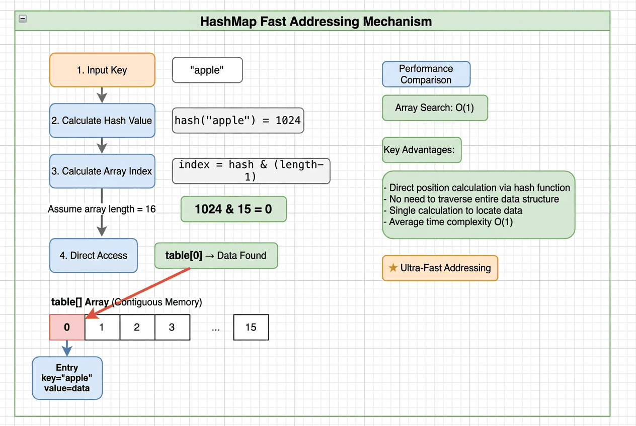Step-by-step HashMap addressing: hash the key, compute the array index, jump directly to the bucket, and resolve locally — achieving O(1) lookup without traversal

Take put("apple", 100) as an example. The entire lookup takes four steps — no full-table scan:

1. Hash the key: Pass the key through a hash function → hash("apple") = 93029210
2. Map to an array index: 93029210 & (arrayLength - 1) → e.g., 93029210 & 15 = 10
3. Jump to the bucket: Access table[10] directly — a single memory access, not a traversal
4. Resolve locally: If no collision, read or write immediately. If there’s a collision, check a small linked list or red-black tree within that bucket.

Why Is HashMap Lookup O(1)?

Array access is O(1) because of a simple addressing formula:

element_address = base_address + index × element_size

Given an index, the memory address is computed with one multiplication and one addition. The cost is fixed regardless of array size — one computation, one memory read. A linked list, by contrast, must be traversed node by node, following pointers through separate memory locations: O(n) in the worst case.

A HashMap hashes a key into an array index, turning what would be a traversal into a computed address. Instead of searching for data, it computes exactly where the data lives and jumps there.

How Does Addressing Change in Distributed Systems?

HashMap solves addressing within a single machine, where data lives in memory and access costs are trivial. At larger scales, the constraints shift dramatically:

Scale Factor	Impact
Data size	Megabytes → terabytes or petabytes across clusters
Storage medium	Memory → disk → network → object storage
Access latency	Memory: ~100 ns / Disk: 10–20 ms / Same-DC network: ~0.5 ms / Cross-region: ~150 ms

The addressing problem doesn’t change — it just gets more expensive. Every lookup may involve network hops and disk I/O, so reducing the number of accesses matters far more than in memory.

To see how real systems handle this, we’ll look at two classic examples. HDFS applies computation-based addressing to large, block-based files. Kafka applies it to append-only message streams. Both follow the same principle: compute where the data is instead of searching for it.

HDFS: Addressing Large Files with In-Memory Metadata

HDFS is a distributed storage system designed for very large files across clusters of machines. Given a file path and byte offset, it needs to find the right data block and the DataNode that stores it.

HDFS solves this with a deliberate design choice: keep all filesystem metadata in memory.

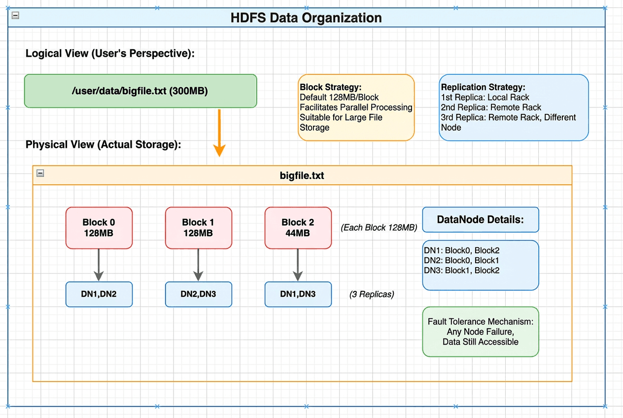HDFS data organization showing logical view of a 300MB file mapped to physical storage as three blocks distributed across DataNodes with replication

At the center is the NameNode. It loads the entire filesystem tree — directory structure, file-to-block mappings, and block-to-DataNode mappings — into memory. Because metadata never touches disk during reads, HDFS resolves all addressing questions through in-memory lookups only.

Conceptually, this is HashMap at cluster scale: use in-memory data structures to turn slow searches into fast, computed lookups. The difference is that HDFS applies the same principle to datasets spread across thousands of machines.

// Data structures stored in the NameNode's memory

// 1. Filesystem directory tree
class FSDirectory {
    INodeDirectory rootDir;           // root directory "/"
    INodeMap inodeMap;                // path → INode (HashMap!)
}

// 2. INode：file / directory node
abstract class INode {
    long id;                          // unique identifier
    String name;                      // name
    INode parent;                     // parent node
    long modificationTime;            // last modification time
}

class INodeFile extends INode {
    BlockInfo[] blocks;               // list of blocks that make up the file
}

// 3. Block metadata mapping
class BlocksMap {
    GSet<Block, BlockInfo> blocks;    // Block → location info (HashMap!)
}

class BlockInfo {
    long blockId;
    DatanodeDescriptor[] storages;    // list of DataNodes storing this block
}

How Does HDFS Locate Data?

Consider reading data at the 200 MB offset of /user/data/bigfile.txt, with a default block size of 128 MB:

1. The client sends a single RPC to the NameNode
2. The NameNode resolves the file path and computes that offset 200 MB falls in the second block (128–256 MB range) — entirely in memory
3. The NameNode returns the DataNodes storing that block (e.g., DN2 and DN3)
4. The client reads directly from the nearest DataNode (DN2)

Total cost: one RPC, a few in-memory lookups, one data read. Metadata never hits disk during this process, and each lookup is constant-time. HDFS avoids expensive metadata scans even as data scales across large clusters.

Apache Kafka: How Sparse Indexing Avoids Random I/O

Apache Kafka is designed for high-throughput message streams. Given a message offset, it needs to locate the exact byte position on disk — without turning reads into random I/O.

Kafka combines sequential storage with a sparse, in-memory index. Instead of searching through data, it computes an approximate location and performs a small, bounded scan.

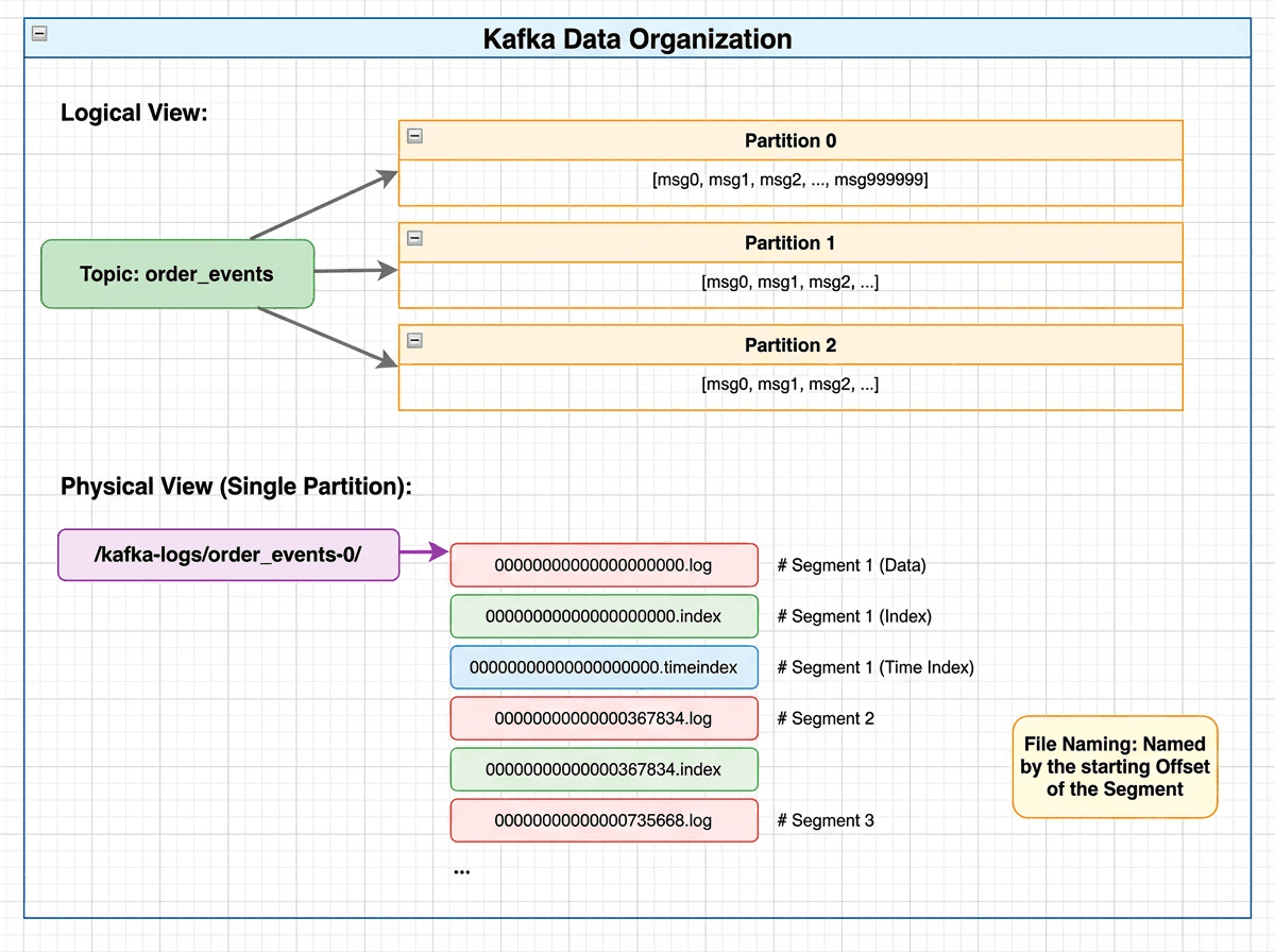Kafka data organization showing logical view with topics and partitions mapped to physical storage as partition directories containing .log, .index, and .timeindex segment files

Messages are organized as Topic → Partition → Segment. Each partition is an append-only log split into segments, each consisting of:

• A .log file storing messages sequentially on disk
• A .index file acting as a sparse index into the log

The .index file is memory-mapped (mmap), so index lookups are served directly from memory without disk I/O.

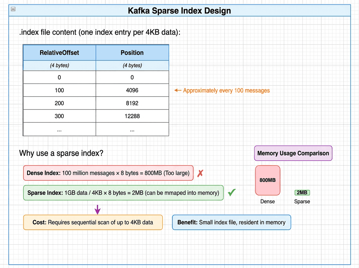Kafka sparse index design showing one index entry per 4KB of data, with memory comparison: dense index at 800MB versus sparse index at just 2MB resident in memory

// A Partition manages all its Segments
class LocalLog {
    // Core structure: TreeMap, ordered by baseOffset
    ConcurrentNavigableMap<Long, LogSegment> segments;

    // Locate the target Segment
    LogSegment floorEntry(long offset) {
        return segments.floorEntry(offset);  // O(log N)
    }
}

// A single Segment
class LogSegment {
    FileRecords log;           // .log file (message data)
    LazyIndex<OffsetIndex> offsetIndex;  // .index file (sparse index)
    long baseOffset;           // starting Offset
}

// Sparse index entry (8 bytes per entry)
class OffsetPosition {
    int relativeOffset;        // offset relative to baseOffset (4 bytes)
    int position;              // physical position in the .log file (4 bytes)
}

How Does Kafka Locate Data?

Suppose a consumer reads the message at offset 500,000. Kafka resolves this in three steps:

1. Locate the segment (TreeMap lookup)

• Segment base offsets: [0, 367834, 735668, 1103502]
• floorEntry(500000) → baseOffset = 367834
• Target file: 00000000000000367834.log
• Time complexity: O(log S), where S is the number of segments (typically < 100)

2. Look up the position in the sparse index (.index)

• Relative offset: 500000 − 367834 = 132166
• Binary search in .index: find the largest entry ≤ 132166 → [132100 → position 20500000]
• Time complexity: O(log N), where N is the number of index entries

3. Sequential read from the log (.log)

• Start reading from position 20,500,000
• Continue until offset 500,000 is reached
• At most one index interval (~4 KB) is scanned

Total: one in-memory segment lookup, one index lookup, one short sequential read. No random disk access.

HDFS vs. Apache Kafka

Dimension	HDFS	Kafka
Design goal	Efficient storage and reading of massive files	High-throughput sequential read/write of message streams
Addressing model	Path → block → DataNode via in-memory HashMaps	Offset → segment → position via sparse index + sequential scan
Metadata storage	Centralized in NameNode memory	Local files, memory-mapped via mmap
Access cost per lookup	1 RPC + N block reads	1 index lookup + 1 data read
Key optimization	All metadata in memory — no disk in the lookup path	Sparse indexing + sequential layout avoids random I/O

Why Object Storage Changes the Addressing Problem

From HashMap to HDFS and Kafka, we’ve seen addressing in memory and in classic distributed storage. As workloads evolve, the requirements keep rising:

• Richer queries. Modern systems handle multi-field filters, similarity search, and complex predicates — not just simple keys and offsets.
• Object storage as the default. Data increasingly lives in S3-compatible stores. Files are spread across buckets, and each access is an API call with fixed latency on the order of tens of milliseconds — even for a few kilobytes.

At this point, latency — not bandwidth — is the bottleneck. A single S3 GET request costs ~50 ms regardless of how much data it returns. If a query triggers thousands of such requests, total latency balloons. Minimizing API fan-out becomes the central design constraint.

We’ll look at two modern systems — Milvus, a vector database, and Apache Iceberg, a lakehouse table format — to see how they address these challenges. Despite their differences, both apply the same core ideas: minimize high-latency accesses, reduce fan-out early, and favor computation over traversal.

Milvus V1: When Field-Level Storage Creates Too Many Files

Milvus is a widely used vector database designed for similarity search over vector embeddings. Its early storage design reflects a common first approach to building on object storage: store each field separately.

In V1, each field in a collection is stored in separate binlog files across segments.

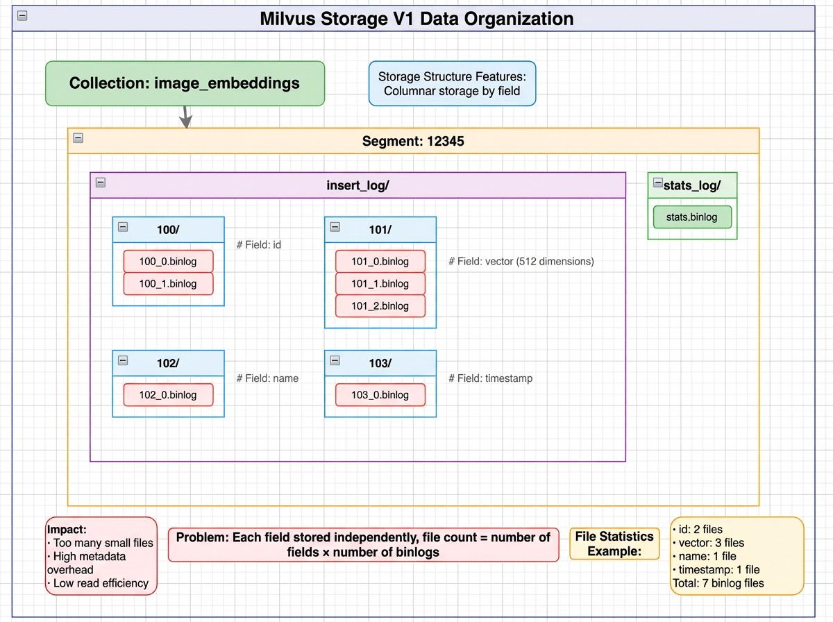Milvus V1 storage layout showing a collection split into segments, with each segment storing fields like id, vector, and scalar data in separate binlog files, plus separate stats_log files for file statistics

How Does Milvus V1 Locate Data?

Consider a simple query: SELECT id, vector FROM collection WHERE id = 123.

1. Metadata lookup — Query etcd/MySQL for the segment list → [Segment 12345, 12346, 12347, …]
2. Read the id field across segments — For each segment, read the id binlog files
3. Locate the target row — Scan loaded id data to find id = 123
4. Read the vector field — Read the corresponding vector binlog files for the matching segment

Total file accesses: N × (F₁ + F₂ + …) where N = number of segments, F = binlog files per field.

The math gets ugly fast. For a collection with 100 fields, 1,000 segments, and 5 binlog files per field:

1,000 × 100 × 5 = 500,000 files

Even if a query touches only three fields, that’s 15,000 object storage API calls. At 50 ms per S3 request, serialized latency reaches 750 seconds — over 12 minutes for a single query.

Milvus V2: How Segment-Level Parquet Cuts API Calls by 10x

To fix the scalability limits in V1, Milvus V2 makes a fundamental change: organize data by segment instead of by field. Rather than many small binlog files, V2 consolidates data into segment-based Parquet files.

The file count drops from N × fields × binlogs to approximately N (one file group per segment).

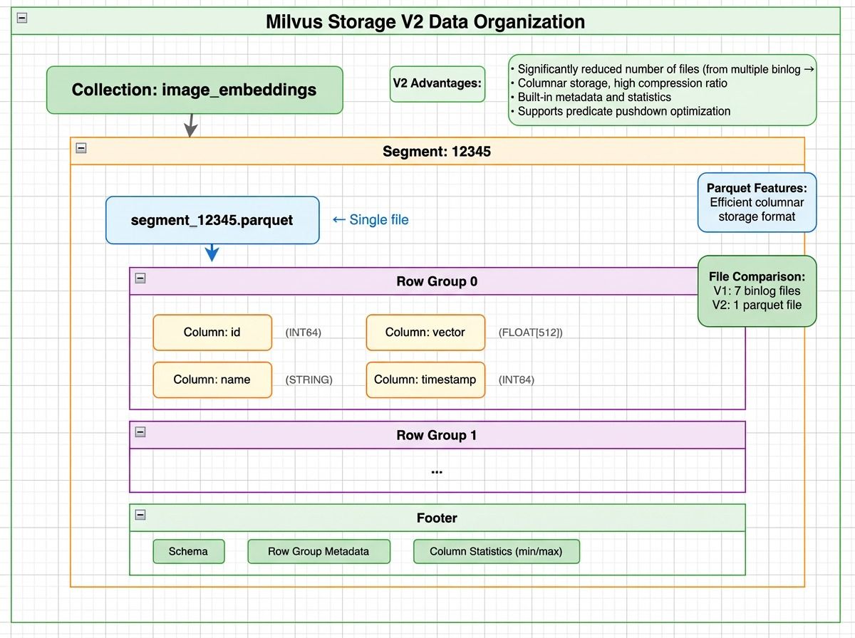Milvus V2 storage layout showing a segment stored as Parquet files with row groups containing column chunks for id, vector, and timestamp, plus a footer with schema and column statistics

But V2 doesn’t store all fields in a single file. It groups fields by size:

• Small scalar fields (like id, timestamp) are stored together
• Large fields (like dense vectors) are split into dedicated files

All files belong to the same segment, and rows are aligned by index across files.

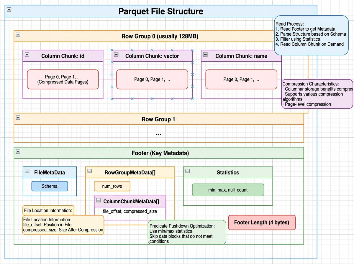Parquet file structure showing row groups with column chunks and compressed data pages, plus a footer containing file metadata, row group metadata, and column statistics like min/max values

How Does Milvus V2 Locate Data?

For the same query — SELECT id, vector FROM collection WHERE id = 123:

1. Metadata lookup — Fetch the segment list → [12345, 12346, …]
2. Read Parquet footers — Extract row group statistics. Check the min/max of the id column per row group. id = 123 falls in Row Group 0 (min=1, max=1000).
3. Read only what’s needed — Parquet’s column pruning reads only the id column from the small-field file and only the vector column from the large-field file. Only matching row groups are accessed.

Splitting large fields out delivers two key benefits:

• More efficient reads. Vector embeddings dominate storage size. Mixed with small fields, they limit how many rows fit in a row group, increasing file accesses. Isolating them lets small-field row groups hold far more rows while large fields use layouts optimized for their size.
• Flexible schema evolution. Adding a column means creating a new file. Removing one means skipping it at read time. No historical data rewrite needed.

The result: file counts drop by more than 10x, API calls by over 10x, and query latency falls from minutes to seconds.

Milvus V1 vs. V2

Aspect	V1	V2
File organization	Split by field	Integrated by segment
Files per collection	N × fields × binlogs	~N × column groups
Storage format	Custom binlog	Parquet (also supports Lance and Vortex)
Column pruning	Natural (field-level files)	Parquet column pruning
Statistics	Separate stats_log files	Embedded in Parquet footer
S3 API calls per query	10,000+	~1,000
Query latency	Minutes	Seconds

Apache Iceberg: Metadata-Driven File Pruning

Apache Iceberg manages analytical tables over massive datasets in lakehouse systems. When a table spans thousands of data files, the challenge is narrowing a query to just the relevant files — without scanning everything.

Iceberg’s answer: decide which files to read before any data I/O happens, using layered metadata. This is the same principle behind metadata filtering in vector databases — use precomputed statistics to skip irrelevant data.

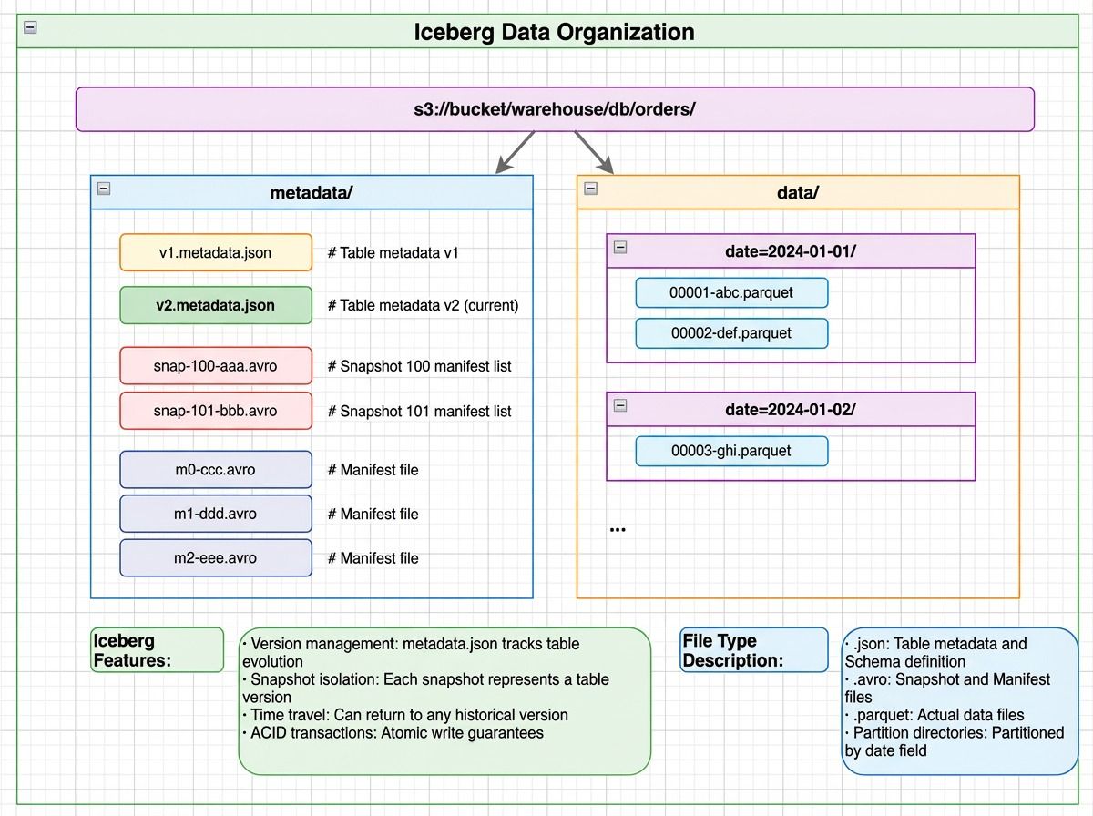Iceberg data organization showing a metadata directory with metadata.json, manifest lists, and manifest files alongside a data directory with date-partitioned Parquet files

Iceberg uses a layered metadata structure. Each layer filters out irrelevant data before the next is consulted — similar in spirit to how distributed databases separate metadata from data for efficient access.

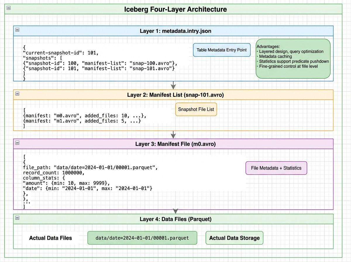Iceberg four-layer architecture: metadata.json points to manifest lists, which reference manifest files containing file-level statistics, which point to actual Parquet data files

How Does Iceberg Locate Data?

Consider: SELECT * FROM orders WHERE date='2024-01-15' AND amount>1000.

1. Read metadata.json (1 I/O) — Load the current snapshot and its manifest lists
2. Read the manifest list (1 I/O) — Apply partition-level filters to skip entire partitions (e.g., all 2023 data is eliminated)
3. Read manifest files (2 I/O) — Use file-level statistics (min/max date, min/max amount) to eliminate files that can’t match the query
4. Read data files (3 I/O) — Only three files remain and are actually read

Instead of scanning all 1,000 data files, Iceberg completes the lookup in 7 I/O operations — avoiding over 94% of unnecessary reads.

How Different Systems Address Data

System	Data Organization	Core Addressing Mechanism	Access Cost
HashMap	Key → array slot	Hash function → direct index	O(1) memory access
HDFS	Path → block → DataNode	In-memory HashMaps + block calculation	1 RPC + N block reads
Kafka	Topic → Partition → Segment	TreeMap + sparse index + sequential scan	1 index lookup + 1 data read
Milvus V2	Collection → Segment → Parquet columns	Metadata lookup + column pruning	N reads (N = segments)
Iceberg	Table → Snapshot → Manifest → Data files	Layered metadata + statistical pruning	3 metadata reads + M data reads

Three Principles Behind Efficient Data Addressing

1. Computation Always Beats Search

Across every system we’ve examined, the most effective optimization follows the same rule: compute where the data is instead of searching for it.

• HashMap computes an array index from hash(key) instead of scanning
• HDFS computes the target block from a file offset instead of traversing filesystem metadata
• Kafka computes the relevant segment and index position instead of scanning the log
• Iceberg uses predicates and file-level statistics to compute which files are worth reading

Computation is arithmetic with a fixed cost. Search is traversal — comparisons, pointer chasing, or I/O — and its cost grows with data size. When a system can derive a location directly, scanning becomes unnecessary.

2. Minimize High-Latency Accesses

This brings us back to the core formula: Total addressing cost = metadata accesses + data accesses. Every optimization ultimately aims at reducing these high-latency operations.

Pattern	Example
Reduce file counts to limit API fan-out	Milvus V2 segment consolidation
Use statistics to rule out data early	Iceberg manifest pruning
Cache metadata in memory	HDFS NameNode, Kafka mmap indexes
Trade small sequential scans for fewer random reads	Kafka sparse index

3. Statistics Enable Early Decisions

Recording simple information at write time — min/max values, partition boundaries, row counts — lets systems decide at read time which files are worth reading and which can be skipped entirely.

This is a small investment with a large payoff. Statistics turn file access from a blind read into a deliberate choice. Whether it’s Iceberg’s manifest-level pruning or Milvus V2’s Parquet footer statistics, the principle is the same: a few bytes of metadata at write time can eliminate thousands of I/O operations at read time.

Conclusion

From Two Sum to HashMap, and from HDFS and Kafka to Milvus and Apache Iceberg, one pattern keeps repeating: performance depends on how efficiently a system locates data.

As data grows and storage moves from memory to disk to object storage, the mechanics change — but the core ideas don’t. The best systems compute locations instead of searching, keep metadata close, and use statistics to avoid touching data that doesn’t matter. Every performance win we’ve examined comes from reducing high-latency accesses and narrowing the search space as early as possible.

Whether you’re designing a vector search pipeline, building systems over unstructured data, or optimizing a lakehouse query engine, the same equation applies. Understanding how your system addresses data is the first step toward making it faster.

---

If you’re working with Milvus and want to optimize your storage or query performance, we’d love to help:

• Join the Milvus Slack community to ask questions, share your architecture, and learn from other engineers working on similar problems.
• Book a free 20-minute Milvus Office Hours session to walk through your use case — whether it’s storage layout, query tuning, or scaling to production.
• If you’d rather skip the infrastructure setup, Zilliz Cloud (managed Milvus) offers a free tier to get started.

---

A few questions that come up when engineers start thinking about data addressing and storage design:

Q: Why did Milvus switch from field-level to segment-level storage?

In Milvus V1, each field was stored in separate binlog files across segments. For a collection with 100 fields and 1,000 segments, this created hundreds of thousands of small files — each requiring its own S3 API call. V2 consolidates data into segment-based Parquet files, reducing file counts by more than 10x and cutting query latency from minutes to seconds. The core insight: on object storage, the number of API calls matters more than total data volume.

Q: How does Milvus handle both vector search and scalar filtering efficiently?

Milvus V2 stores scalar fields and vector fields in separate file groups within the same segment. Scalar queries use Parquet column pruning and row group statistics to skip irrelevant data. Vector search uses dedicated vector indexes. Both share the same segment structure, so hybrid queries — combining scalar filters with vector similarity — can operate on the same data without duplication.

Q: Does the “computation over search” principle apply to vector databases?

Yes. Vector indexes like HNSW and IVF are built on the same idea. Instead of comparing a query vector against every stored vector (brute-force search), they use graph structures or cluster centroids to compute approximate neighborhoods and jump directly to relevant regions of the vector space. The tradeoff — a small accuracy loss for orders-of-magnitude fewer distance computations — is the same “computation over search” pattern applied to high-dimensional embedding data.

Q: What’s the biggest performance mistake teams make with object storage?

Creating too many small files. Each S3 GET request has a fixed latency floor (~50 ms), regardless of how much data it returns. A system that reads 10,000 small files serializes 500 seconds of latency — even if total data volume is modest. The fix is consolidation: merge small files into larger ones, use columnar formats like Parquet for selective reads, and maintain metadata that lets you skip files entirely.