

MinHash LSH finds near-duplicate documents without comparing every pair. MinHash turns each document’s set of shingles (overlapping word or character n-grams) into a short fixed-length signature whose positions agree with probability equal to the Jaccard similarity of the two sets. Locality-sensitive hashing (LSH) then splits each signature into bands and hashes each band into buckets, so only documents that collide in at least one band become candidates. In Milvus, the MINHASH_LSH index on a BINARY_VECTOR field with the MHJACCARD metric implements this, which makes it practical to deduplicate LLM training corpora, crawled web pages, and document collections with millions or billions of items.
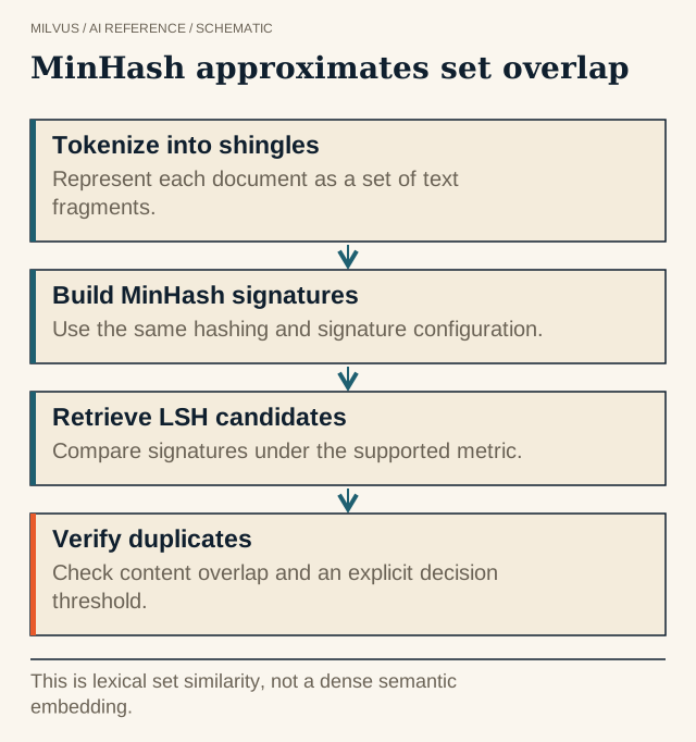 MinHash approximates set overlap. This is lexical set similarity, not a dense semantic embedding.
Why not just compare every pair?
Near-duplicate detection is usually framed as: find all pairs of documents whose Jaccard similarity J(A, B) = |A ∩ B| / |A ∪ B| exceeds a threshold, where A and B are the documents’ shingle sets. Computing it exactly for every pair is quadratic. One million documents produce about 500 billion pairs, and real pretraining corpora are thousands of times larger. Exact hashing (an MD5 of the normalized text) is cheap but only catches byte-identical copies, missing pages that differ by a timestamp, a footer, or a few edited sentences.
MinHash LSH gives you a cheap, tunable approximation: you trade a small chance of missing a pair, and some false candidates, for near-linear work.
How does MinHash estimate Jaccard similarity?
Andrei Broder introduced MinHash in 1997 to remove duplicate pages from AltaVista’s search results. The steps are:
- Normalize and shingle. Lowercase, strip punctuation or boilerplate as needed, then break the text into shingles. With 3-word shingles, “the quick brown fox” yields
{the quick brown, quick brown fox}. - Hash with many functions. Apply
nindependent hash functions to every shingle. - Keep the minimum. For each hash function, record the smallest hash value over all shingles. The
nminimums form the signature.
The key property: for a random hash function, the probability that two sets have the same minimum equals their Jaccard similarity. So the fraction of matching positions across the signature is an unbiased estimate of J, and its error shrinks roughly as 1/√n. With 256 hash functions, the standard error is a few percentage points, and each document is represented by a fixed-size signature no matter how long it is.
Shingle choices change what “duplicate” means. Word shingles of size 1 to 3 are typical and depend on a language-aware tokenizer; character shingles of 2 to 6 work for any language and are more sensitive to small edits. Larger shingles make the measure stricter about word order. Treat normalization, shingle type, shingle size, and hash count as part of a versioned representation, because changing any of them changes every similarity score.
How does LSH banding find candidates?
Even with signatures, comparing all pairs is still quadratic. LSH avoids it:
- Split each
n-value signature intobbands ofrvalues, son = b × r. - Hash each band to a bucket.
- Two documents become a candidate pair if they land in the same bucket for at least one band.
If two documents have Jaccard similarity s, the chance they agree on all r values in a band is s^r, and the chance they collide in at least one of b bands is:
P(candidate) = 1 − (1 − s^r)^b
This produces an S-shaped curve with a steep rise near s ≈ (1/b)^(1/r). Pairs well above that point almost always collide; pairs well below almost never do.
| Bands × rows (n) | Approx. threshold | P at s = 0.3 | P at s = 0.5 | P at s = 0.7 | P at s = 0.8 |
|---|---|---|---|---|---|
| 64 × 2 (128) | 0.12 | 0.998 | ~1.0 | ~1.0 | ~1.0 |
| 32 × 4 (128) | 0.42 | 0.23 | 0.87 | >0.999 | ~1.0 |
| 16 × 8 (128) | 0.71 | 0.001 | 0.06 | 0.61 | 0.95 |
More bands with fewer rows raise recall and the number of candidates; fewer bands with more rows raise precision and cut candidates. Pick the shape so the steep part of the curve sits just below the similarity you consider a duplicate, then verify candidates.
MinHash LSH vs semantic deduplication
MinHash measures surface overlap: shared shingles. It catches copies with light edits, reformatting, or reordered sections, and it is cheap and explainable. It does not catch paraphrases or translations, because those share few shingles. Embedding-based deduplication measures meaning and catches paraphrases, but it is more expensive and more prone to merging documents that are on the same topic but genuinely different. Many data pipelines run exact hashing first, MinHash LSH second, and embedding similarity (for example a range search with a high threshold) as an optional third pass. The deduplication guide covers how to combine them.
MinHash LSH in Milvus
Milvus stores MinHash signatures as binary vectors and indexes them with MINHASH_LSH. Requirements:
- The vector field must be
BINARY_VECTOR, withdimequal tonum_hashes × bits per hash value. index_typeisMINHASH_LSH(orBIN_FLATfor exact comparison).metric_typemust beMHJACCARD, a metric specific to MinHash signatures. PlainJACCARD,L2, orCOSINEgive wrong results here.
Generating signatures. You can compute signatures yourself (for example with the datasketch library or a Spark job) and insert them as bytes, or, in Milvus 3.0, let Milvus generate them with the built-in MinHash function. The function reads a VARCHAR field with enable_analyzer=True and writes a BINARY_VECTOR whose dim is 32 × num_hashes:
from pymilvus import Function, FunctionType, DataType

schema.add_field("content", DataType.VARCHAR, max_length=9000, enable_analyzer=True)
schema.add_field("signature", DataType.BINARY_VECTOR, dim=32 * 256)

schema.add_function(Function(
    name="minhash",
    function_type=FunctionType.MINHASH,
    input_field_names=["content"],
    output_field_names=["signature"],
    params={"num_hashes": 256, "shingle_size": 3, "token_level": "word"},
))

index_params = client.prepare_index_params()
index_params.add_index(
    field_name="signature",
    index_type="MINHASH_LSH",
    metric_type="MHJACCARD",
    params={"mh_element_bit_width": 32, "mh_lsh_band": 32},
)
The function also accepts token_level="char" for language-agnostic character shingles, a hash_function of xxhash (default) or sha1, and a seed. When signatures come from this function, mh_element_bit_width must be 32.
Key index parameters.
| Parameter | What it does |
|---|---|
mh_element_bit_width | Bits per hash value: 8, 16, 32, or 64. Must match how signatures were produced. |
mh_lsh_band | Number of bands b; must divide the signature length evenly. Docs suggest starting at 32 bands for a 128-value signature, raising it for recall or lowering it for speed. |
with_raw_data | Store the full signatures alongside LSH codes so candidates can be rescored. |
mh_lsh_bloom_false_positive_prob | False-positive rate for the Bloom filter used in bucket lookups, 0.001 to 0.1. |
Search parameters. By default a search returns LSH candidates ranked by estimated similarity. Setting mh_search_with_jaccard=True (with with_raw_data enabled at build time) computes a more exact Jaccard score on the candidates, and refine_k sets how many candidates are rescored. Use refinement whenever results drive deletions.
A common streaming pattern is search before insert: for each incoming document, search the collection for neighbors above your threshold, and insert only if none are found.
Calibrating before you delete anything
Approximate candidates can include pairs that fail your duplicate rule, and the banding can miss some true pairs. Before applying a policy at scale:
- Label a sample covering exact copies, formatting changes, boilerplate-heavy pages, partial overlaps, translations, and genuinely different documents.
- Measure candidate recall (true duplicates found) and false removals separately while sweeping
mh_lsh_band, shingle size, and the final threshold. - Watch for chaining when you group pairs into clusters: A can match B and B can match C even when A and C are quite different. Decide whether clusters keep one representative per connected component or need a stricter rule.
- Run in report-only mode first and export a manifest of proposed removals with IDs and scores, so the decision is reviewable and reversible.
- Check downstream impact, including whether rare domains or languages were disproportionately removed.
For broader context on dataset cleaning, see what is data curation. To build the pipeline end to end, start Milvus with the Quickstart and follow the MINHASH_LSH guide.


