

Batching several query vectors into one request usually raises throughput, because the database amortizes per-request overhead and can share work across queries, but it raises the latency each individual query sees, because every query in the batch waits for the slowest one and for the batch to fill. Batching helps offline jobs such as bulk scoring, deduplication, and evaluation. It hurts interactive search, where a user waiting for one answer pays for the whole batch. The useful goal is the highest throughput that still meets your tail-latency target.
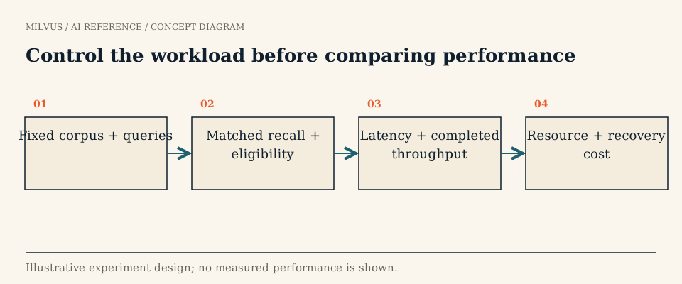 Control the workload before comparing performance
Latency vs. throughput: the definitions
Latency is the time from sending a request to receiving its result, best reported as percentiles (p50, p95, p99) because users notice the slow tail. Throughput is completed queries per second (QPS). The two are linked by Little’s law: the average number of requests in flight equals arrival rate times average time in the system.
An illustrative example: at 200 QPS with an average latency of 50 ms, about 200 × 0.05 = 10 requests are in flight at any moment. If latency rises to 100 ms at the same arrival rate, 20 are in flight. When a resource saturates, latency climbs, more requests pile up, and latency climbs further. That feedback loop is why tail latency explodes near saturation even though average throughput looks fine.
Batching vs. concurrency: what’s the difference?
They are easy to confuse, and databases treat them differently.
- A batch is one request carrying several query vectors. In Milvus you pass a list of vectors in
data, and Milvus runs the ANN searches for them in parallel and returns one result list per query vector. - Concurrency is several independent requests in flight at once, typically from many users or threads.
# One request, three query vectors (a batch, nq = 3)
res = client.search(
    collection_name="docs",
    anns_field="embedding",
    data=[q1, q2, q3],
    limit=10,
    search_params={"params": {"ef": 64}},
)
for hits in res:   # one result list per query vector
    ...
A batch shares one network round trip, one request parse, and one scheduling decision, and lets the engine work on the queries side by side. Concurrency gives the scheduler independent work it can interleave, which keeps latency per user low until CPU, memory bandwidth, or disk I/O runs out.
When does batching help, and when does it hurt?
| Scenario | Batch? | Why |
|---|---|---|
| Offline evaluation, bulk deduplication, nightly recommendations | Yes, large batches | Only total completion time matters |
| GPU indexes such as GPU_CAGRA | Yes | GPUs need many parallel queries to stay busy |
| Multi-query retrieval for one user request (query rewrites, multi-vector) | Yes, small batch | The queries are needed together anyway |
| Interactive search, chat, autocomplete | No, or very small | Waiting to fill a batch adds directly to user latency |
| Mixed online and offline traffic on one cluster | Separate them | Large batches can starve interactive queries |
Two costs are easy to miss. Accumulation delay: if a server-side or client-side batcher waits up to 20 ms to collect queries, every query in that batch pays up to 20 ms extra before search even starts. Result size: a batch of 100 queries at top-k 100 returns 10,000 hits, and returning large output_fields with each hit can make serialization and network transfer dominate. Milvus caps a single ANN search at a limit plus offset below 16,384 results; use search iterators beyond that.
How do you find the saturation point?
- Fix everything that affects work per query: dataset, index, search parameters, top-k, filters, output fields, and the consistency level.
- Measure serially first, one request at a time, for best-case latency.
- Increase concurrency in steps (1, 2, 4, 8, 16, …). At each step record QPS, p50, p99, and errors.
- Plot throughput and p99 against concurrency. Throughput rises roughly linearly, then flattens. Where it flattens, p99 starts to climb steeply. That knee is the saturation point.
- Repeat with batch sizes you might use (nq = 1, 10, 100) to see how batching moves the knee.
- Check the client. A single-threaded Python load generator can become the bottleneck long before the database does. Watch its CPU too.
VectorDBBench automates much of this, reporting serial p99 latency and maximum QPS across concurrency levels. The benchmarking guide covers the rest of the methodology.
Which Milvus settings move the numbers?
- Search parameters.
effor HNSW,nprobefor IVF, andsearch_listfor DISKANN set how much of the index each query explores. Lower values cut latency and raise throughput, at the cost of recall. Always change them against a fixed recall target. See HNSW tuning. - Index type. Graph indexes generally deliver the highest throughput at a given recall; IVF variants can be preferable when top-k is very large or filters are very selective, according to the Milvus index guide. See choosing an index.
- In-memory replicas. Loading a collection with more replicas spreads reads over more query nodes, which raises the throughput ceiling and improves failover. It does not make a single query faster, and each replica holds a full copy of the segments, so memory scales with replica count.
- Memory placement. Data fully in RAM gives the most predictable tail. mmap lets a node hold more data than RAM, with latency close to in-memory as long as the working set fits in page cache, and degrading when it does not. The mmap guide compares it with disk-based indexes.
- Consistency level. Strong reads can wait for query nodes to catch up with recent writes, which shows up as extra latency under heavy ingest. Use it only on requests that need read-after-write.
- Filters and output fields. Selective metadata filters change the amount of graph traversal; large output fields add transfer time.
Change one setting at a time, re-measure at the same recall, and keep the curve. When traffic grows you will know which lever to pull next.
Measuring end-to-end latency
The database is often not the slowest step. A typical RAG request also includes query embedding, network hops, reranking, and fetching source documents. Instrument each stage separately so you tune the step that actually dominates. Count requests that time out or fail as part of the result: a configuration that reports great latency because it dropped the slow requests has not met the target.
Related reading
- How should you benchmark vector search performance?
- What is GPU_CAGRA, and when does it help vector search?
- How do you locate a bottleneck across Milvus components?
- How do vector databases support recommendation candidate retrieval?
Start with the Milvus Quickstart and the vector search reference, then turn your target QPS into a hardware estimate with the Milvus sizing tool. If you would rather scale replicas and capacity without managing nodes, Zilliz Cloud runs managed Milvus.


