

An IVF (inverted file) index speeds up vector search by clustering the dataset with k-means and searching only the clusters closest to the query. Each cluster is represented by its centroid, and every stored vector is filed in an “inverted list” under its nearest centroid. At query time the index compares the query with the centroids, picks the nprobe closest clusters, and scans only the vectors in those lists. Two parameters matter most: nlist, the number of clusters built, and nprobe, the number searched per query.
IVF describes how candidates are narrowed down, not how vectors are stored. That is why Milvus offers several IVF variants, such as IVF_FLAT, IVF_SQ8, IVF_PQ, and IVF_RABITQ, which share the same clustering step but keep different representations inside each list.
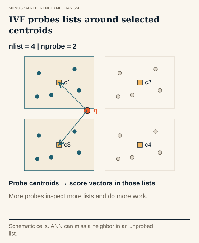 IVF centroid and region selection
How does an IVF index work, step by step?
1. Train the coarse quantizer. The index runs k-means on the vectors (or a sample of them) to find nlist centroids. Together, the centroids split the vector space into Voronoi cells: every point in the space belongs to the cell of whichever centroid is nearest.
2. Assign and store. Every vector is assigned to its nearest centroid and appended to that centroid’s list. The name comes from text search, where an inverted index maps a term to the documents containing it; here a centroid maps to the vectors in its cell.
3. Probe at query time. The query is compared with all nlist centroids, which is cheap because nlist is small compared with the dataset. The nprobe nearest cells are selected.
4. Scan the selected lists. Distances are computed between the query and every vector in those lists, and the best k are returned. With IVF_FLAT these are exact distances on the original vectors; with compressed variants they are approximations.
The only approximation in plain IVF_FLAT comes from step 3. If a true nearest neighbor sits in a cell that was not probed, it is missed. This happens most often near cell boundaries: a query close to the edge of its cell may have its nearest neighbor just across the line, in a neighboring cell whose centroid is a little farther away. Raising nprobe fixes this by covering more neighboring cells.
Why is IVF faster than brute force?
A brute-force scan computes N distances per query. With IVF, assuming roughly balanced clusters, a query computes nlist centroid distances plus about N × nprobe / nlist vector distances. For 10 million vectors with nlist = 4,096 and nprobe = 16, that is about 4,096 + 39,000 distance computations instead of 10 million, roughly a 250x reduction in work. Real clusters are never perfectly balanced, so some queries touch larger lists than others, which shows up as variance in tail latency.
How do nlist and nprobe affect recall and speed?
| Change | Effect on recall | Effect on latency and cost |
|---|---|---|
Raise nprobe | Higher, because more neighboring cells are covered | Linear increase in vectors scanned |
Raise nlist (same nprobe) | Lower, because each probed cell is smaller | Fewer vectors scanned per query; longer k-means training |
Raise nlist and nprobe together | Similar recall with finer cells | Often a better speed/recall balance on large data, with more centroid comparisons |
The ratio nprobe / nlist is the fraction of the data a query scans, and it is the best single predictor of both recall and cost. A widely used starting heuristic is nlist somewhere between √N and 4√N for N vectors, then a sweep of nprobe to find the recall target. Treat it as a starting point: clustered or skewed data may need different values.
In Milvus, indexes are built per sealed segment rather than over the whole collection at once, so N in that heuristic is the number of vectors in a segment, not the collection total.
IVF parameters in Milvus
According to the Milvus guides for IVF_FLAT, IVF_SQ8, and IVF_PQ:
| Parameter | Stage | Range | Default | Notes |
|---|---|---|---|---|
nlist | Build | [1, 65536] | 128 | Docs recommend 32 to 4,096 |
nprobe | Search | [1, nlist] | 8 | Main recall/latency knob |
m | Build, IVF_PQ only | [1, 65536] | none | Number of sub-vectors; must divide the dimension |
nbits | Build, IVF_PQ only | [1, 24] | 8 | Bits per sub-vector code (2^nbits centroids per sub-space) |
All three support L2, IP, and COSINE. Building and searching an IVF_FLAT index:
from pymilvus import MilvusClient

client = MilvusClient(uri="http://localhost:19530")

index_params = client.prepare_index_params()
index_params.add_index(
    field_name="embedding",
    index_type="IVF_FLAT",
    metric_type="COSINE",
    params={"nlist": 1024},
)
client.create_index(collection_name="docs", index_params=index_params)

res = client.search(
    collection_name="docs",
    anns_field="embedding",
    data=[query_vector],
    limit=10,
    search_params={"params": {"nprobe": 32}},
)
Because nprobe is a search parameter, you can raise it for a high-recall offline job and lower it for an interactive path, all on the same index.
IVF_FLAT, IVF_SQ8, IVF_PQ, or IVF_RABITQ?
The variants differ in what is stored inside each inverted list:
- IVF_FLAT stores full float32 vectors. Distances inside probed cells are exact, so recall depends only on
nprobe. Memory is roughly the raw data size. - IVF_SQ8 maps each dimension to one byte by scaling it into the 0 to 255 range. Vectors take about a quarter of the space, and recall usually drops only slightly.
- IVF_PQ splits each vector into
msub-vectors and stores a codebook ID for each. A 768-dimensional vector withm = 96andnbits = 8takes 96 bytes instead of 3,072. That is a 32x reduction, with more recall loss and some tuning effort. - IVF_RABITQ stores roughly one bit per dimension and corrects the estimate with refinement. It is covered in What is IVF_RABITQ?.
Compression adds a second, separate source of error. When recall is low, first check coverage by raising nprobe on IVF_FLAT. If IVF_FLAT reaches the target and the compressed variant does not, the gap is quantization error, not cell coverage. The quantization guide explains how SQ and PQ codes are formed.
When does IVF beat HNSW, and when not?
IVF builds faster than HNSW, because k-means plus assignment is cheaper than inserting every vector into a graph, and it adds almost no structural memory beyond the centroids. Its compressed variants are the most straightforward way to fit a large corpus into limited RAM. HNSW, in return, usually reaches high recall at lower latency and keeps that recall more steadily as search effort is reduced, whereas IVF recall can fall off quickly once nprobe stops covering the cells that hold the true neighbors.
Two IVF weaknesses are worth knowing. Centroids are learned from the data present at build time, so a large shift in the data (a new embedding model, a new content domain) leaves cells unbalanced until the index is rebuilt. And when filters exclude most vectors, many probed cells contain few eligible matches, so you may need a larger nprobe to return k results; see the metadata filtering guide. For a side-by-side decision across all index families, use how to choose a vector index. GPU variants (GPU_IVF_FLAT, GPU_IVF_PQ) are compared with CAGRA in the GPU_CAGRA guide.
How should you tune an IVF index?
- Compute exact ground truth for a representative query set with a FLAT baseline.
- Build IVF_FLAT with an
nlistnear the heuristic for your segment size. - Sweep
nprobe(for example 1, 4, 8, 16, 32, 64) and plot Recall@k against p95 latency. - If you need the same recall at lower cost, try a different
nlistas a separate build experiment. - Only then swap in IVF_SQ8 or IVF_PQ and compare at the same recall, recording memory, build time, and tail latency.
Change one thing at a time. If you change nlist, nprobe, and the quantizer together, you cannot tell which one moved the result.
You can run this whole sequence locally with the Milvus Quickstart, or on Zilliz Cloud if you would rather not operate the cluster yourself.


